Machine Learning
Summary and Key Takeaways
Core Principles
Generalization: The ultimate goal is to create models that perform well on unseen data, not just the training data.
Bias-Variance Tradeoff: Every model makes a tradeoff between underfitting (high bias) and overfitting (high variance).
No Free Lunch: No single algorithm works best for all problems. Choose based on your data and problem characteristics.
Feature Engineering: The quality of your features often matters more than the choice of algorithm.
Evaluation: Always use proper evaluation techniques (train-test split, cross-validation) to assess model performance.
Practical Skills Acquired
Data preprocessing and cleaning
Exploratory data analysis and visualization
Feature engineering and selection
Model selection and hyperparameter tuning
Supervised learning (classification and regression)
Unsupervised learning (clustering, dimensionality reduction)
Neural networks and deep learning
Model evaluation and interpretation
Python programming with ML libraries (numpy, pandas, scikit-learn, tensorflow/keras)
Python Libraries Used
| Library | Purpose | Key Functions/Classes |
|---|---|---|
| numpy | Numerical computing | array, linspace, random, etc. |
| pandas | Data manipulation | DataFrame, Series, read_csv, etc. |
| matplotlib | Visualization | pyplot, figure, scatter, plot, etc. |
| seaborn | Statistical visualization | heatmap, boxplot, pairplot, etc. |
| scikit-learn | Machine learning | All ML algorithms, preprocessing, metrics |
| tensorflow/keras | Deep learning | Sequential, Dense, Conv2D, etc. |
| librosa | Audio processing | load, stft, mfcc, etc. |
Quick Reference
Common Preprocessing Steps
# 1. Load data
import pandas as pd
from sklearn.ensemble import RandomForestClassifier
from sklearn.utils._repr_html import estimator
from zmq.backend import backend

df = pd.read_csv('machine-learning/DiabetesDataset.csv')

# 2. Handle missing values
df['Glucose'] = df['Glucose'].fillna(df['Glucose'].mean())  # Numerical
df['SkinThickness'] = df['SkinThickness'].fillna(df['SkinThickness'].mode())  # Categorical
df.dropna(inplace=True) # Simply drop rows with missing values

# 3. Encode categorical variables
from sklearn.preprocessing import OneHotEncoder
encoder = OneHotEncoder(drop='first', sparse_output=False)
X_encoded = encoder.fit_transform(df[['Diabetes']])

# 4. Scale numerical features
from sklearn.preprocessing import StandardScaler
scaler = StandardScaler()
X_scaled = scaler.fit_transform(df.select_dtypes(include=['float64', 'int64']))
y = df['Diabetes']

# 5. Train-test split
from sklearn.model_selection import train_test_split
X_train, X_test, y_train, y_test = train_test_split(X_scaled, y, test_size=0.2, random_state=42)
Common Hyperparameter Tuning
from sklearn.model_selection import GridSearchCV, RandomizedSearchCV
from scipy.stats import randint

# Grid Search
param_grid = {'n_estimators': [50, 100, 200], 'max_depth': [None, 10, 20], 'min_samples_split': [2, 5, 10]}
grid_search = GridSearchCV(estimator, param_grid, cv=5, scoring='accuracy')
grid_search.fit(X_train, y_train)
print(f"Best parameters: {grid_search.best_params_}")
print(f"Best score: {grid_search.best_score_:.4f}")

# Random Search
param_dist = {'n_estimators': randint(50, 200), 'max_depth': [None] + list(randint(5, 50).rvs(10)), 'min_samples_split': randint(2, 20)}
random_search = RandomizedSearchCV(estimator, param_dist, n_iter=20, cv=5)
random_search.fit(X_train, y_train)
Output
Best parameters: {'max_depth': None, 'min_samples_split': 2, 'n_estimators': 50}
Best score: 1.0000
Common Model Evaluation
from sklearn.metrics import (
    accuracy_score, precision_score, recall_score, f1_score,
    confusion_matrix, classification_report,
    mean_squared_error, mean_absolute_error, r2_score
)

estimator = RandomForestClassifier(min_samples_split=2, n_estimators=50, max_depth=None, random_state=42)
estimator.fit(X_train, y_train)
y_pred = estimator.predict(X_test)

# Classification metrics
print(f"Accuracy: {accuracy_score(y_test, y_pred):.4f}")
print(f"Precision: {precision_score(y_test, y_pred):.4f}")
print(f"Recall: {recall_score(y_test, y_pred):.4f}")
print(f"F1: {f1_score(y_test, y_pred):.4f}")
print(f"Confusion Matrix:\n{confusion_matrix(y_test, y_pred)}")
print(f"Classification Report:\n{classification_report(y_test, y_pred)}")

# Regression metrics
print(f"MSE: {mean_squared_error(y_test, y_pred):.4f}")
print(f"MAE: {mean_absolute_error(y_test, y_pred):.4f}")
print(f"R²: {r2_score(y_test, y_pred):.4f}")
Output
Accuracy: 1.0000
Precision: 1.0000
Recall: 1.0000
F1: 1.0000
Confusion Matrix:
[[99  0]
 [ 0 55]]
Classification Report:
              precision    recall  f1-score   support

           0       1.00      1.00      1.00        99
           1       1.00      1.00      1.00        55

    accuracy                           1.00       154
   macro avg       1.00      1.00      1.00       154
weighted avg       1.00      1.00      1.00       154

MSE: 0.0000
MAE: 0.0000
R²: 1.0000
Introduction to Machine Learning
Educational Objectives
Basic, high-level understanding of what machine learning is
Understand the three main ML paradigms with examples
Data preparation and visualization techniques
Identify different data types and their characteristics
Perform data consolidation, preprocessing, and cleaning
Create effective data visualizations
Key Concepts
ML Paradigms
Data: where is input, is label Goal: Learn function to map Example: Classifying apples vs. oranges
Data: (no labels) Goal: Learn underlying structure in data Example: Grouping similar items together
Data: State-action pairs Goal: Maximize future rewards over time Example: Learning to navigate an environment
Data Types
| Type | Description | Example |
|---|---|---|
| Numerical | Continuous or discrete numbers | Age, temperature |
| Categorical | Finite set of categories | Color, gender |
| Ordinal | Categories with order | Rating (1-5 stars) |
| Text | Natural language | Product reviews |
| Image | Pixel arrays | Photographs |
| Audio | Sound waveforms | Speech recordings |
Data Preprocessing Pipeline
Practical Example: Data Visualization
import pandas as pd
import matplotlib.pyplot as plt
import seaborn as sns
# Load data
data = pd.read_csv('machine-learning/DiabetesDataset.csv')
# Basic visualization
plt.figure(figsize=(10, 6))
sns.boxplot(data=data.select_dtypes(include=['float64', 'int64']))
plt.title('Feature Distribution')
plt.xticks(rotation=45)
plt.show()
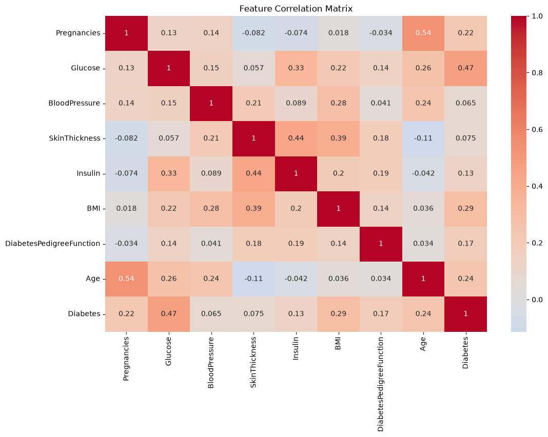
# Correlation matrix
plt.figure(figsize=(12, 8))
sns.heatmap(data.corr(), annot=True, cmap='coolwarm', center=0)
plt.title('Feature Correlation Matrix')
plt.show()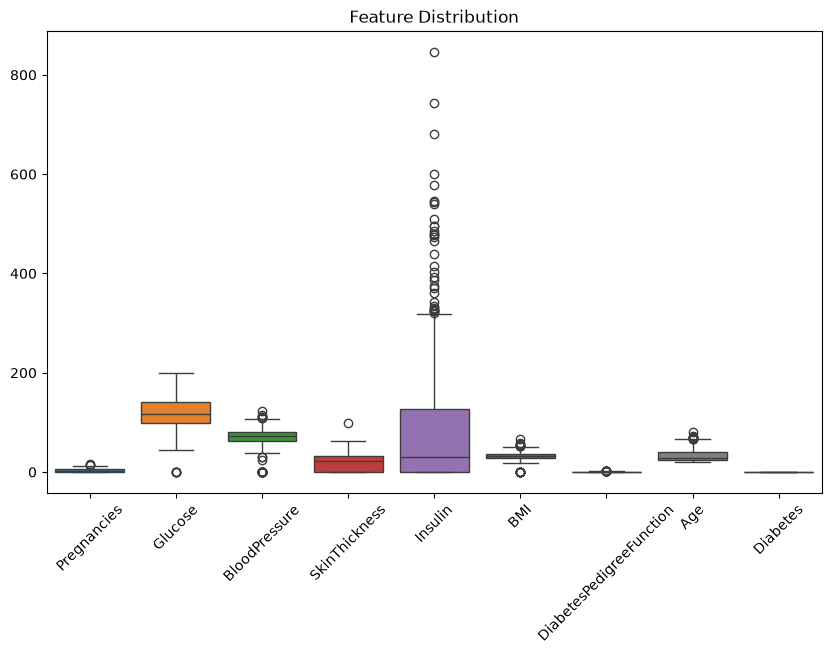
Supervised Learning & k-Nearest Neighbors
Educational Objectives
Address supervised ML problems: outline approach and name main concepts
Understand and explain the kNN algorithm and its advantages/disadvantages
Remember and explain most frequently used distance measures
Remember and explain prevalent performance measures for ML evaluation
Key Concepts
k-Nearest Neighbors Algorithm
kNN is a simple, instance-based learning algorithm:
Store all training data
Calculate distance between new point and all training points
Find k nearest neighbors
Predict based on majority vote (classification) or average (regression)
Choosing k
Small k: More flexible, can overfit, sensitive to noise
Large k: More stable, can underfit, smoother decision boundaries
Optimal k: Found via cross-validation
Distance Measures
| Measure | Formula | When to Use |
|---|---|---|
| Euclidean | General purpose | |
| Manhattan | High-dimensional data | |
| Cosine | Text data | |
| Hamming | Count of differing positions | Categorical data |
Performance Measures
Accuracy:
Precision: (How many selected are correct?)
Recall: (How many actual positives found?)
F1 Score:
Confusion Matrix: Visualizes TP, TN, FP, FN
MSE: Mean Squared Error - sensitive to outliers
RMSE: Root Mean Squared Error - same units as target
MAE: Mean Absolute Error - robust to outliers
R²: Coefficient of determination - explains variance
import numpy as np

# rows := actual, cols := predicted
confusion_matrix = np.array([
    [12, 6, 9],   # Actual Yellow Car
    [8, 14, 2],   # Actual Green Car
    [3, 1, 7]     # Actual Blue Car
])

tp = confusion_matrix[1, 1]
fp = confusion_matrix[:, 1].sum() - tp
fn = confusion_matrix[1, :].sum() - tp
tn = confusion_matrix.sum() - (tp + fp + fn)

precision = tp / (tp + fp)
recall = tp / (tp + fn)
f1 = 2 * (precision * recall) / (precision + recall)

print(f"Accuracy: {tp + tn / (tp + tn + fp + fn):.4f}")
print(f"Precision: {precision:.4f}")
print(f"Recall: {recall:.4f}")
print(f"F1: {f1:.4f}")
Accuracy: 14.5000
Precision: 0.6667
Recall: 0.5833
F1: 0.6222
Practical Example: kNN Implementation
from sklearn.neighbors import KNeighborsClassifier
from sklearn.model_selection import train_test_split
from sklearn.metrics import accuracy_score, classification_report
from sklearn.preprocessing import StandardScaler

# Load and prepare data
df = pd.read_csv('machine-learning/DiabetesDataset.csv')
X = df.drop('Diabetes', axis=1)
y = df['Diabetes']
X_train, X_test, y_train, y_test = train_test_split(
    X, y, test_size=0.2, random_state=42
)

# Scale features (important for distance-based algorithms)
scaler = StandardScaler()
X_train_scaled = scaler.fit_transform(X_train)
X_test_scaled = scaler.transform(X_test)

# Train kNN classifier
knn = KNeighborsClassifier(n_neighbors=5, metric='euclidean')
knn.fit(X_train_scaled, y_train)

# Make predictions
y_pred = knn.predict(X_test_scaled)

# Evaluate
print(f"Accuracy: {accuracy_score(y_test, y_pred):.4f}")
print(classification_report(y_test, y_pred))

# Find optimal k using cross-validation
from sklearn.model_selection import GridSearchCV
param_grid = {'n_neighbors': range(1, 21)}
grid_search = GridSearchCV(knn, param_grid, cv=5)
grid_search.fit(X_train_scaled, y_train)
print(f"Best k: {grid_search.best_params_['n_neighbors']}")
Output
Accuracy: 0.6948
              precision    recall  f1-score   support

           0       0.75      0.80      0.77        99
           1       0.58      0.51      0.54        55

    accuracy                           0.69       154
   macro avg       0.66      0.65      0.66       154
weighted avg       0.69      0.69      0.69       154

Best k: 11
Model Selection, Bias-Variance Tradeoff & Regularization
Educational Objectives
Understand the No Free Lunch theorem and Ockham’s Razor
Explain the influence of bias and variance on model performance
Explain loss minimization with stochastic gradient descent (SGD)
Use sound experimental setup to select model parameters, evaluate models, and choose among models
Key Concepts
Bias-Variance Tradeoff
Regularization Techniques
| Technique | Formula | Effect |
|---|---|---|
| Lasso (L1) | Feature selection, sparse weights | |
| Ridge (L2) | Prevents large weights | |
| Elastic Net | Combines L1 and L2 |
Model Evaluation
Notebook Cell
import pandas as pd
from sklearn.ensemble import RandomForestClassifier

df = pd.read_csv('machine-learning/DiabetesDataset.csv')
X = df.drop('Diabetes', axis=1)
y = df['Diabetes']

estimator = RandomForestClassifier(random_state=42)
Train-Test Split
from sklearn.model_selection import train_test_split

X_train, X_test, y_train, y_test = train_test_split(
    X, y, test_size=0.2, random_state=42, stratify=y
)
K-Fold Cross-Validation
from sklearn.model_selection import cross_val_score, KFold


kfold = KFold(n_splits=5, shuffle=True, random_state=42)
cv_scores = cross_val_score(estimator, X, y, cv=kfold, scoring='accuracy')
print(f"Mean CV Accuracy: {cv_scores.mean():.4f} (+/- {cv_scores.std() * 2:.4f})")
Mean CV Accuracy: 0.7643 (+/- 0.0488)
Learning Curves
from sklearn.model_selection import learning_curve
import matplotlib.pyplot as plt
import numpy as np

train_sizes, train_scores, test_scores = learning_curve(
    estimator, X, y, cv=5, train_sizes=np.linspace(0.1, 1.0, 10)
)
plt.figure(figsize=(10, 6))
plt.plot(train_sizes, train_scores.mean(1), 'o-', label='Training score')
plt.plot(train_sizes, test_scores.mean(1), 'o-', label='Cross-validation score')
plt.xlabel('Training examples')
plt.ylabel('Score')
plt.legend()
plt.title('Learning Curve')
plt.show()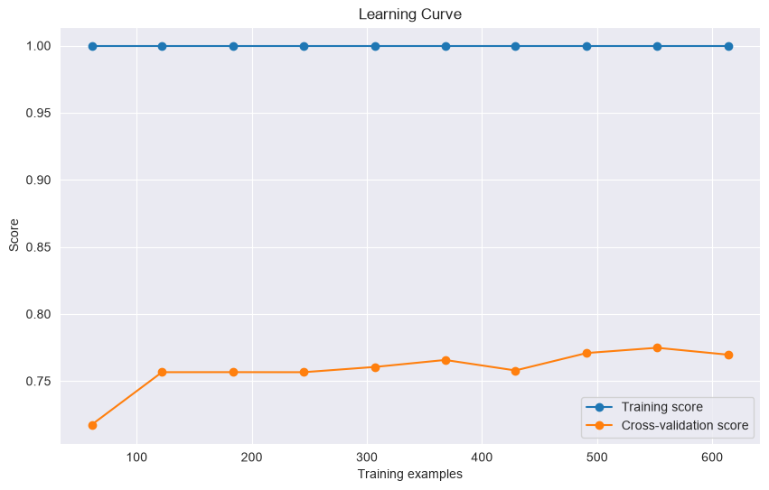
from sklearn.linear_model import SGDClassifier, SGDRegressor
sgd_clf = SGDClassifier(loss='log_loss', penalty='l2', alpha=0.0001, max_iter=1000, random_state=42)
sgd_reg = SGDRegressor(penalty='l2', alpha=0.0001, max_iter=1000, random_state=42)
Feature Engineering
Educational Objectives
Use EDA, data preparation, and cleaning as necessary steps before ML projects
Generate features using transformations (binning, interaction features)
Explain four approaches for feature selection
Generate features from text data (BoW, tf-idf, n-grams)
Identify important features for audio data: STFT and MFCC
Key Concepts
Feature Engineering Pipeline
Data Cleaning
import pandas as pd
import matplotlib.pyplot as plt
import seaborn as sns

# Load data
df = pd.read_csv('machine-learning/DiabetesDataset.csv')

# Handle missing values
df.dropna(inplace=True)

# Handle outliers using IQR
def remove_outliers(df, column):
    Q1 = df[column].quantile(0.25)
    Q3 = df[column].quantile(0.75)
    IQR = Q3 - Q1
    lower_bound = Q1 - 1.5 * IQR
    upper_bound = Q3 + 1.5 * IQR
    return df[(df[column] >= lower_bound) & (df[column] <= upper_bound)]


fig, (ax1, ax2) = plt.subplots(1, 2, figsize=(12, 5), sharey=True)
ax1.set_title('Before')
ax2.set_title('After')

sns.boxplot(data=df['Insulin'], ax=ax1)
df = remove_outliers(df, 'Insulin')
sns.boxplot(data=df["Insulin"], ax=ax2)
<Axes: title={'center': 'After'}, ylabel='Insulin'>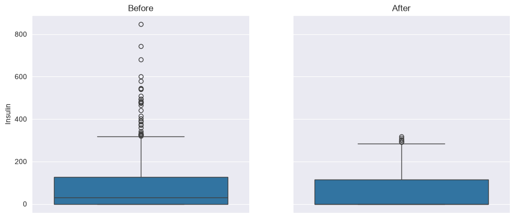
Feature Generation Techniques
Binning: Convert continuous to categorical
Polynomial: for non-linear relationships
Interaction: for feature combinations
Log Transform: for skewed distributions
Scaling: Standardize or normalize features
One-Hot Encoding: Create binary columns for each category
Label Encoding: Convert categories to integers
Target Encoding: Replace categories with target mean
Frequency Encoding: Replace with frequency of category
from sklearn.preprocessing import StandardScaler, MinMaxScaler, RobustScaler, OneHotEncoder, PolynomialFeatures

# Load data
X = pd.read_csv('machine-learning/DiabetesDataset.csv')

# Standard scaling
scaler = StandardScaler()
X_scaled = scaler.fit_transform(X)

# Min-max scaling
minmax = MinMaxScaler()
X_minmax = minmax.fit_transform(X)

# Robust scaling
robust = RobustScaler()
X_robust = robust.fit_transform(X)

# One-hot encoding
encoder = OneHotEncoder(drop='first', sparse_output=False)
X_encoded = encoder.fit_transform(X)

# Polynomial features
poly = PolynomialFeatures(degree=2, include_bias=False)
X_poly = poly.fit_transform(X)
Text Feature Extraction
Counts word occurrences
Ignores grammar and word order
Simple and effective baseline
Term Frequency-Inverse Document Frequency
Weights words by importance
Rare words get higher weights
from sklearn.feature_extraction.text import CountVectorizer, TfidfVectorizer

texts = np.array([
    'The sun is shining',
    'The weather is sweet',
    'The sun is shining and the weather is sweet'
])

# Bag of Words
bow = CountVectorizer(max_features=1000, stop_words='english', ngram_range=(1, 2))
X_bow = bow.fit_transform(texts)

# TF-IDF
tfidf = TfidfVectorizer(max_features=1000, stop_words='english', ngram_range=(1, 2))
X_tfidf = tfidf.fit_transform(texts)
Audio Feature Extraction
Converts audio to time-frequency representation
Captures frequency content over time
Useful for speech and music analysis
Represents spectral envelope of sound
Mimics human auditory system
State-of-the-art for speech recognition
import librosa

# Load audio file
y, sr = librosa.load('machine-learning/0_george_1.wav', sr=22050)

# Extract STFT
stft = librosa.stft(y, n_fft=2048, hop_length=512)
stft_magnitude = np.abs(stft)

# Extract MFCC
mfccs = librosa.feature.mfcc(y=y, sr=sr, n_mfcc=13)
mfcc_mean = np.mean(mfccs, axis=1)
mfcc_std = np.std(mfccs, axis=1)
Output
---------------------------------------------------------------------------
ImportError                               Traceback (most recent call last)
Cell In[37], line 4
      1 import librosa
      2
      3 # Load audio file
----> 4 y, sr = librosa.load('machine-learning/0_george_1.wav', sr=22050)
      5
      6 # Extract STFT
      7 stft = librosa.stft(y, n_fft=2048, hop_length=512)

File ~/Development/marbetschar/marco.betschart.name/.venv/lib/python3.12/site-packages/lazy_loader/__init__.py:79, in attach.<locals>.__getattr__(name)
     77 submod_path = f"{package_name}.{attr_to_modules[name]}"
     78 submod = importlib.import_module(submod_path)
---> 79 attr = getattr(submod, name)
     81 # If the attribute lives in a file (module) with the same
     82 # name as the attribute, ensure that the attribute and *not*
     83 # the module is accessible on the package.
     84 if name == attr_to_modules[name]:

File ~/Development/marbetschar/marco.betschart.name/.venv/lib/python3.12/site-packages/lazy_loader/__init__.py:78, in attach.<locals>.__getattr__(name)
     76 elif name in attr_to_modules:
     77     submod_path = f"{package_name}.{attr_to_modules[name]}"
---> 78     submod = importlib.import_module(submod_path)
     79     attr = getattr(submod, name)
     81     # If the attribute lives in a file (module) with the same
     82     # name as the attribute, ensure that the attribute and *not*
     83     # the module is accessible on the package.

File /opt/homebrew/Cellar/python@3.12/3.12.10_1/Frameworks/Python.framework/Versions/3.12/lib/python3.12/importlib/__init__.py:90, in import_module(name, package)
     88             break
     89         level += 1
---> 90 return _bootstrap._gcd_import(name[level:], package, level)

File <frozen importlib._bootstrap>:1387, in _gcd_import(name, package, level)

File <frozen importlib._bootstrap>:1360, in _find_and_load(name, import_)

File <frozen importlib._bootstrap>:1334, in _find_and_load_unlocked(name, import_)

File <frozen importlib._bootstrap>:950, in _load_unlocked(spec)

File <frozen importlib._bootstrap_external>:999, in _LoaderBasics.exec_module(self, module)

File <frozen importlib._bootstrap>:488, in _call_with_frames_removed(f, *args, **kwds)

File ~/Development/marbetschar/marco.betschart.name/.venv/lib/python3.12/site-packages/librosa/core/audio.py:18
     15 import soxr
     16 import lazy_loader as lazy
---> 18 from numba import jit, stencil, guvectorize
     19 from .fft import get_fftlib
     20 from .convert import frames_to_samples, time_to_samples

File ~/Development/marbetschar/marco.betschart.name/.venv/lib/python3.12/site-packages/numba/__init__.py:59
     54             msg = ("Numba requires SciPy version 1.0 or greater. Got SciPy "
     55                    f"{scipy.__version__}.")
     56             raise ImportError(msg)
---> 59 _ensure_critical_deps()
     60 # END DO NOT MOVE
     61 # ---------------------- WARNING WARNING WARNING ----------------------------
     64 from ._version import get_versions

File ~/Development/marbetschar/marco.betschart.name/.venv/lib/python3.12/site-packages/numba/__init__.py:45, in _ensure_critical_deps()
     42 if numpy_version > (2, 4):
     43     msg = (f"Numba needs NumPy 2.4 or less. Got NumPy "
     44            f"{numpy_version[0]}.{numpy_version[1]}.")
---> 45     raise ImportError(msg)
     47 try:
     48     import scipy

ImportError: Numba needs NumPy 2.4 or less. Got NumPy 2.5.
Feature Selection Methods
| Method | Description | When to Use |
|---|---|---|
| Variance Threshold | Remove features with low variance | Initial filtering |
| Univariate Selection | Select best features based on statistical tests | Quick feature reduction |
| RFE | Remove features iteratively based on model weights | Model-based selection |
| Model-based Ranking | Use feature importance from models | Tree-based models |
import pandas as pd
from sklearn.linear_model import LogisticRegression
from sklearn.feature_selection import VarianceThreshold, SelectKBest, RFE, f_classif

df = pd.read_csv('machine-learning/DiabetesDataset.csv')
X = df.drop('Diabetes', axis=1)
y = df['Diabetes']

# Variance threshold
selector = VarianceThreshold(threshold=0.01)
X_selected = selector.fit_transform(X)

# Select top k features
selector = SelectKBest(score_func=f_classif, k=3)
X_selected = selector.fit_transform(X, y)

# Recursive Feature Elimination
estimator = LogisticRegression(max_iter=1000)
selector = RFE(estimator, n_features_to_select=5)
X_selected = selector.fit_transform(X, y)
Linear Models & Logistic Regression
Educational Objectives
Understand probability theory fundamentals (random variables, distributions)
Design loss functions using maximum likelihood and negative log-likelihood
Implement logistic regression for binary classification
Understand neuron structure and activation functions
Key Concepts
Probability Theory Basics
Bernoulli: Binary outcomes (p)
Gaussian: Continuous, symmetric (μ, σ²)
Multinomial: Multiple categories
Poisson: Count data (λ)
Loss Function Design
Maximum Likelihood Estimation (MLE)
Negative Log-Likelihood (NLL)
Logistic Regression
Sigmoid Function
Binary Cross-Entropy Loss
Implementation
from sklearn.linear_model import LogisticRegression, LogisticRegressionCV
from sklearn.metrics import accuracy_score, confusion_matrix, precision_score, recall_score, f1_score
from sklearn.model_selection import train_test_split

df = pd.read_csv('machine-learning/DiabetesDataset.csv')
X = df.drop('Diabetes', axis=1)
y = df['Diabetes']

X_train, X_test, y_train, y_test = train_test_split(X, y, test_size=0.2, random_state=42)

# Basic logistic regression
model = LogisticRegression(penalty='l2', C=1.0, solver='lbfgs', max_iter=1000, random_state=42)
model.fit(X_train, y_train)

# Logistic regression with cross-validated regularization
model_cv = LogisticRegressionCV(Cs=[0.001, 0.01, 0.1, 1, 10, 100], cv=5, penalty='l2', solver='lbfgs', max_iter=1000, random_state=42)
model_cv.fit(X_train, y_train)

# Get coefficients
feature_importance = pd.DataFrame({'Feature': X.columns, 'Coefficient': model.coef_[0]}).sort_values('Coefficient', ascending=False)

# Predictions and evaluation
y_pred = model.predict(X_test)
y_proba = model.predict_proba(X_test)

print(f"Accuracy: {accuracy_score(y_test, y_pred):.4f}")
print(f"Precision: {precision_score(y_test, y_pred):.4f}")
print(f"Recall: {recall_score(y_test, y_pred):.4f}")
print(f"F1 Score: {f1_score(y_test, y_pred):.4f}")
confusion_matrix(y_test, y_pred)
Accuracy: 0.7468
Precision: 0.6379
Recall: 0.6727
F1 Score: 0.6549
array([[78, 21],
       [18, 37]])
Neural Networks & Deep Learning
Educational Objectives
Understand neural network architectures (shallow and deep)
Explain activation functions (ReLU, sigmoid, softmax)
Understand loss functions (MSE, cross-entropy)
Implement training with gradient descent and backpropagation
Apply optimization techniques (momentum, adaptive learning rates)
Implement CNNs for image processing
Apply regularization (L1/L2, dropout) and hyperparameter tuning
Key Concepts
Neural Network Architecture
Activation Functions
Function: Pros: Solves vanishing gradient, computationally efficient Cons: Dies for negative inputs
Function: Pros: Outputs between 0 and 1 Cons: Vanishing gradients
Function: Use: Multi-class classification output Property: Outputs sum to 1
Loss Functions
| Loss Function | Formula | Use Case |
|---|---|---|
| MSE | Regression | |
| Binary Cross-Entropy | Binary classification | |
| Categorical Cross-Entropy | Multi-class classification |
Backpropagation
Forward pass: Compute predictions and loss
Backward pass: Compute gradients using chain rule
Update weights: Adjust weights using gradients
Optimization Techniques
Update:
Update:
Adaptive learning rates for each parameter
Combines momentum and adaptive learning rates
Regularization Techniques
L1: - Encourages sparsity
L2: - Prevents large weights
Elastic Net: Combination of both
Randomly deactivate neurons during training Prevents co-adaptation of neurons Typical rate: 0.2-0.5 for hidden layers
Practical Example: Neural Network with Keras
import matplotlib.pyplot as plt

from tensorflow import keras
from tensorflow.keras import layers
from tensorflow.keras.callbacks import EarlyStopping

# Load and clean data
df = pd.read_csv('machine-learning/DiabetesDataset.csv')
X = df.drop('Diabetes', axis=1)
y = df['Diabetes']

X_train, X_test, y_train, y_test = train_test_split(X, y, test_size=0.2, random_state=42)
input_dim = X.shape[1]

# Define a simple neural network
model = keras.Sequential([
    layers.Dense(64, activation='relu', input_shape=(input_dim,)),
    layers.BatchNormalization(),
    layers.Dropout(0.3),
    layers.Dense(32, activation='relu'),
    layers.BatchNormalization(),
    layers.Dropout(0.2),
    layers.Dense(1, activation='sigmoid')  # Binary classification
])

# Compile the model
model.compile(optimizer='adam', loss='binary_crossentropy', metrics=['accuracy'])

# Early stopping
early_stopping = EarlyStopping(monitor='val_loss', patience=10, restore_best_weights=True)

# Train the model
history = model.fit(X_train, y_train, validation_data=(X_test, y_test), epochs=100, batch_size=32, callbacks=[early_stopping], verbose=1)

# Plot training history
plt.figure(figsize=(12, 4))
plt.subplot(1, 2, 1)
plt.plot(history.history['accuracy'], label='Training Accuracy')
plt.plot(history.history['val_accuracy'], label='Validation Accuracy')
plt.legend()
plt.title('Accuracy over epochs')

plt.subplot(1, 2, 2)
plt.plot(history.history['loss'], label='Training Loss')
plt.plot(history.history['val_loss'], label='Validation Loss')
plt.legend()
plt.title('Loss over epochs')
plt.show()

# Evaluate
loss, accuracy = model.evaluate(X_test, y_test)
print(f"Test Accuracy: {accuracy:.4f}")
Epoch 1/100
20/20 ━━━━━━━━━━━━━━━━━━━━ 1s 5ms/step - accuracy: 0.6075 - loss: 0.7251 - val_accuracy: 0.3571 - val_loss: 3.6762
Epoch 2/100
20/20 ━━━━━━━━━━━━━━━━━━━━ 0s 2ms/step - accuracy: 0.6922 - loss: 0.6318 - val_accuracy: 0.3571 - val_loss: 2.7727
Epoch 3/100
20/20 ━━━━━━━━━━━━━━━━━━━━ 0s 2ms/step - accuracy: 0.6922 - loss: 0.6022 - val_accuracy: 0.3571 - val_loss: 2.0603
Epoch 4/100
20/20 ━━━━━━━━━━━━━━━━━━━━ 0s 2ms/step - accuracy: 0.7362 - loss: 0.5714 - val_accuracy: 0.3636 - val_loss: 1.6119
Epoch 5/100
20/20 ━━━━━━━━━━━━━━━━━━━━ 0s 2ms/step - accuracy: 0.7182 - loss: 0.6093 - val_accuracy: 0.4026 - val_loss: 1.3522
Epoch 6/100
20/20 ━━━━━━━━━━━━━━━━━━━━ 0s 2ms/step - accuracy: 0.7410 - loss: 0.5509 - val_accuracy: 0.4740 - val_loss: 1.1482
Epoch 7/100
20/20 ━━━━━━━━━━━━━━━━━━━━ 0s 1ms/step - accuracy: 0.7264 - loss: 0.5644 - val_accuracy: 0.5065 - val_loss: 0.9677
Epoch 8/100
20/20 ━━━━━━━━━━━━━━━━━━━━ 0s 1ms/step - accuracy: 0.7476 - loss: 0.5292 - val_accuracy: 0.5844 - val_loss: 0.8118
Epoch 9/100
20/20 ━━━━━━━━━━━━━━━━━━━━ 0s 1ms/step - accuracy: 0.7313 - loss: 0.5377 - val_accuracy: 0.6558 - val_loss: 0.7464
Epoch 10/100
20/20 ━━━━━━━━━━━━━━━━━━━━ 0s 1ms/step - accuracy: 0.7524 - loss: 0.5107 - val_accuracy: 0.6753 - val_loss: 0.7077
Epoch 11/100
20/20 ━━━━━━━━━━━━━━━━━━━━ 0s 1ms/step - accuracy: 0.7508 - loss: 0.5157 - val_accuracy: 0.7013 - val_loss: 0.6539
Epoch 12/100
20/20 ━━━━━━━━━━━━━━━━━━━━ 0s 1ms/step - accuracy: 0.7394 - loss: 0.5104 - val_accuracy: 0.6818 - val_loss: 0.6117
Epoch 13/100
20/20 ━━━━━━━━━━━━━━━━━━━━ 0s 1ms/step - accuracy: 0.7443 - loss: 0.5396 - val_accuracy: 0.6818 - val_loss: 0.5923
Epoch 14/100
20/20 ━━━━━━━━━━━━━━━━━━━━ 0s 1ms/step - accuracy: 0.7476 - loss: 0.5272 - val_accuracy: 0.7143 - val_loss: 0.5663
Epoch 15/100
20/20 ━━━━━━━━━━━━━━━━━━━━ 0s 1ms/step - accuracy: 0.7378 - loss: 0.5084 - val_accuracy: 0.7338 - val_loss: 0.5535
Epoch 16/100
20/20 ━━━━━━━━━━━━━━━━━━━━ 0s 1ms/step - accuracy: 0.7524 - loss: 0.5020 - val_accuracy: 0.7338 - val_loss: 0.5504
Epoch 17/100
20/20 ━━━━━━━━━━━━━━━━━━━━ 0s 1ms/step - accuracy: 0.7524 - loss: 0.5342 - val_accuracy: 0.7468 - val_loss: 0.5392
Epoch 18/100
20/20 ━━━━━━━━━━━━━━━━━━━━ 0s 1ms/step - accuracy: 0.7736 - loss: 0.4804 - val_accuracy: 0.7532 - val_loss: 0.5321
Epoch 19/100
20/20 ━━━━━━━━━━━━━━━━━━━━ 0s 1ms/step - accuracy: 0.7557 - loss: 0.4875 - val_accuracy: 0.7727 - val_loss: 0.5296
Epoch 20/100
20/20 ━━━━━━━━━━━━━━━━━━━━ 0s 1ms/step - accuracy: 0.7524 - loss: 0.4988 - val_accuracy: 0.7662 - val_loss: 0.5310
Epoch 21/100
20/20 ━━━━━━━━━━━━━━━━━━━━ 0s 1ms/step - accuracy: 0.7638 - loss: 0.4951 - val_accuracy: 0.7662 - val_loss: 0.5362
Epoch 22/100
20/20 ━━━━━━━━━━━━━━━━━━━━ 0s 1ms/step - accuracy: 0.7492 - loss: 0.4789 - val_accuracy: 0.7662 - val_loss: 0.5332
Epoch 23/100
20/20 ━━━━━━━━━━━━━━━━━━━━ 0s 1ms/step - accuracy: 0.7736 - loss: 0.4801 - val_accuracy: 0.7597 - val_loss: 0.5457
Epoch 24/100
20/20 ━━━━━━━━━━━━━━━━━━━━ 0s 1ms/step - accuracy: 0.7459 - loss: 0.4987 - val_accuracy: 0.7662 - val_loss: 0.5500
Epoch 25/100
20/20 ━━━━━━━━━━━━━━━━━━━━ 0s 1ms/step - accuracy: 0.7638 - loss: 0.4763 - val_accuracy: 0.7727 - val_loss: 0.5362
Epoch 26/100
20/20 ━━━━━━━━━━━━━━━━━━━━ 0s 1ms/step - accuracy: 0.7492 - loss: 0.4857 - val_accuracy: 0.7792 - val_loss: 0.5280
Epoch 27/100
20/20 ━━━━━━━━━━━━━━━━━━━━ 0s 1ms/step - accuracy: 0.7655 - loss: 0.4602 - val_accuracy: 0.7532 - val_loss: 0.5337
Epoch 28/100
20/20 ━━━━━━━━━━━━━━━━━━━━ 0s 1ms/step - accuracy: 0.7280 - loss: 0.4937 - val_accuracy: 0.7403 - val_loss: 0.5364
Epoch 29/100
20/20 ━━━━━━━━━━━━━━━━━━━━ 0s 1ms/step - accuracy: 0.7524 - loss: 0.5068 - val_accuracy: 0.7597 - val_loss: 0.5356
Epoch 30/100
20/20 ━━━━━━━━━━━━━━━━━━━━ 0s 1ms/step - accuracy: 0.7720 - loss: 0.4679 - val_accuracy: 0.7597 - val_loss: 0.5278
Epoch 31/100
20/20 ━━━━━━━━━━━━━━━━━━━━ 0s 1ms/step - accuracy: 0.7508 - loss: 0.4952 - val_accuracy: 0.7468 - val_loss: 0.5424
Epoch 32/100
20/20 ━━━━━━━━━━━━━━━━━━━━ 0s 1ms/step - accuracy: 0.7427 - loss: 0.5075 - val_accuracy: 0.7338 - val_loss: 0.5455
Epoch 33/100
20/20 ━━━━━━━━━━━━━━━━━━━━ 0s 1ms/step - accuracy: 0.7752 - loss: 0.4666 - val_accuracy: 0.7662 - val_loss: 0.5353
Epoch 34/100
20/20 ━━━━━━━━━━━━━━━━━━━━ 0s 1ms/step - accuracy: 0.7687 - loss: 0.4610 - val_accuracy: 0.7662 - val_loss: 0.5360
Epoch 35/100
20/20 ━━━━━━━━━━━━━━━━━━━━ 0s 1ms/step - accuracy: 0.7785 - loss: 0.4688 - val_accuracy: 0.7597 - val_loss: 0.5303
Epoch 36/100
20/20 ━━━━━━━━━━━━━━━━━━━━ 0s 1ms/step - accuracy: 0.7785 - loss: 0.4726 - val_accuracy: 0.7532 - val_loss: 0.5296
Epoch 37/100
20/20 ━━━━━━━━━━━━━━━━━━━━ 0s 1ms/step - accuracy: 0.7655 - loss: 0.4675 - val_accuracy: 0.7403 - val_loss: 0.5431
Epoch 38/100
20/20 ━━━━━━━━━━━━━━━━━━━━ 0s 1ms/step - accuracy: 0.7736 - loss: 0.4775 - val_accuracy: 0.7468 - val_loss: 0.5474
Epoch 39/100
20/20 ━━━━━━━━━━━━━━━━━━━━ 0s 1ms/step - accuracy: 0.7606 - loss: 0.4761 - val_accuracy: 0.7273 - val_loss: 0.5553
Epoch 40/100
20/20 ━━━━━━━━━━━━━━━━━━━━ 0s 1ms/step - accuracy: 0.7557 - loss: 0.4660 - val_accuracy: 0.7532 - val_loss: 0.5432
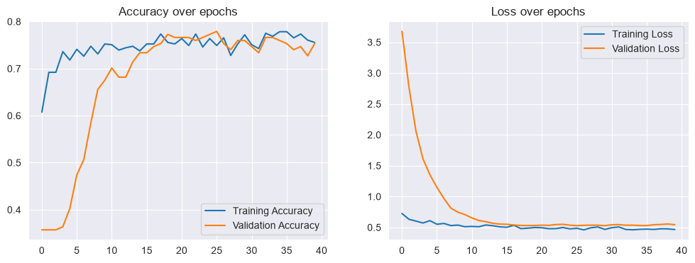
5/5 ━━━━━━━━━━━━━━━━━━━━ 0s 2ms/step - accuracy: 0.7597 - loss: 0.5278
Test Accuracy: 0.7597
Convolutional Neural Networks (CNNs)
Educational Objectives
Understand convolution operations for image processing
Implement pooling layers (max pooling, average pooling)
Apply CNNs to classification, detection, and segmentation tasks
Design CNN architectures for various computer vision tasks
Key Concepts
CNN Architecture Components
Convolution Operation
Kernel size: Typically 3x3, 5x5, 7x7
Stride: Step size of kernel (usually 1)
Padding: ‘same’ or ‘valid’
Number of filters: Determines output depth
Pooling Operations
Takes maximum value in each window Preserves most prominent features Reduces spatial dimensions
Takes average value in each window Smoother than max pooling Less sensitive to outliers
Practical Example: CNN for Fashion MNIST
from tensorflow import keras
from tensorflow.keras import layers
import numpy as np

# Load Fashion MNIST dataset
(x_train, y_train), (x_test, y_test) = keras.datasets.fashion_mnist.load_data()

# Preprocess data
x_train = x_train.astype('float32') / 255.0
x_test = x_test.astype('float32') / 255.0
x_train = np.expand_dims(x_train, -1)  # Shape: (60000, 28, 28, 1)
x_test = np.expand_dims(x_test, -1)    # Shape: (10000, 28, 28, 1)

# Convert labels to one-hot encoding
y_train = keras.utils.to_categorical(y_train, 10)
y_test = keras.utils.to_categorical(y_test, 10)

# Define CNN model
model = keras.Sequential([
    layers.Conv2D(32, kernel_size=(3, 3), activation='relu', input_shape=(28, 28, 1), padding='same'),
    layers.BatchNormalization(),
    layers.MaxPooling2D(pool_size=(2, 2)),
    layers.Dropout(0.3),
    layers.Conv2D(64, kernel_size=(3, 3), activation='relu', padding='same'),
    layers.BatchNormalization(),
    layers.MaxPooling2D(pool_size=(2, 2)),
    layers.Dropout(0.4),
    layers.Conv2D(128, kernel_size=(3, 3), activation='relu', padding='same'),
    layers.BatchNormalization(),
    layers.MaxPooling2D(pool_size=(2, 2)),
    layers.Dropout(0.5),
    layers.Flatten(),
    layers.Dense(128, activation='relu'),
    layers.BatchNormalization(),
    layers.Dropout(0.5),
    layers.Dense(10, activation='softmax')  # 10 classes
])

# Compile model
model.compile(optimizer='adam', loss='categorical_crossentropy', metrics=['accuracy'])

# Train model
history = model.fit(x_train, y_train, batch_size=128, epochs=30, validation_split=0.2)

# Evaluate
score = model.evaluate(x_test, y_test, verbose=0)
print(f'Test loss: {score[0]:.4f}')
print(f'Test accuracy: {score[1]:.4f}')
Epoch 1/30
375/375 ━━━━━━━━━━━━━━━━━━━━ 9s 20ms/step - accuracy: 0.7201 - loss: 0.7927 - val_accuracy: 0.5803 - val_loss: 1.3395
Epoch 2/30
375/375 ━━━━━━━━━━━━━━━━━━━━ 7s 19ms/step - accuracy: 0.8252 - loss: 0.4829 - val_accuracy: 0.8673 - val_loss: 0.3565
Epoch 3/30
375/375 ━━━━━━━━━━━━━━━━━━━━ 7s 19ms/step - accuracy: 0.8514 - loss: 0.4158 - val_accuracy: 0.8881 - val_loss: 0.3069
Epoch 4/30
375/375 ━━━━━━━━━━━━━━━━━━━━ 7s 19ms/step - accuracy: 0.8632 - loss: 0.3791 - val_accuracy: 0.8914 - val_loss: 0.2920
Epoch 5/30
375/375 ━━━━━━━━━━━━━━━━━━━━ 7s 20ms/step - accuracy: 0.8726 - loss: 0.3526 - val_accuracy: 0.8910 - val_loss: 0.2916
Epoch 6/30
375/375 ━━━━━━━━━━━━━━━━━━━━ 8s 20ms/step - accuracy: 0.8782 - loss: 0.3383 - val_accuracy: 0.8879 - val_loss: 0.2958
Epoch 7/30
375/375 ━━━━━━━━━━━━━━━━━━━━ 7s 20ms/step - accuracy: 0.8833 - loss: 0.3216 - val_accuracy: 0.9041 - val_loss: 0.2614
Epoch 8/30
375/375 ━━━━━━━━━━━━━━━━━━━━ 8s 22ms/step - accuracy: 0.8867 - loss: 0.3089 - val_accuracy: 0.9098 - val_loss: 0.2435
Epoch 9/30
375/375 ━━━━━━━━━━━━━━━━━━━━ 8s 22ms/step - accuracy: 0.8892 - loss: 0.3019 - val_accuracy: 0.9066 - val_loss: 0.2487
Epoch 10/30
375/375 ━━━━━━━━━━━━━━━━━━━━ 8s 20ms/step - accuracy: 0.8923 - loss: 0.2962 - val_accuracy: 0.9129 - val_loss: 0.2365
Epoch 11/30
375/375 ━━━━━━━━━━━━━━━━━━━━ 8s 20ms/step - accuracy: 0.8966 - loss: 0.2874 - val_accuracy: 0.9133 - val_loss: 0.2377
Epoch 12/30
375/375 ━━━━━━━━━━━━━━━━━━━━ 8s 21ms/step - accuracy: 0.8987 - loss: 0.2824 - val_accuracy: 0.9113 - val_loss: 0.2344
Epoch 13/30
375/375 ━━━━━━━━━━━━━━━━━━━━ 8s 21ms/step - accuracy: 0.8990 - loss: 0.2769 - val_accuracy: 0.8921 - val_loss: 0.2973
Epoch 14/30
375/375 ━━━━━━━━━━━━━━━━━━━━ 8s 22ms/step - accuracy: 0.9016 - loss: 0.2724 - val_accuracy: 0.9198 - val_loss: 0.2170
Epoch 15/30
375/375 ━━━━━━━━━━━━━━━━━━━━ 8s 21ms/step - accuracy: 0.9023 - loss: 0.2705 - val_accuracy: 0.9165 - val_loss: 0.2259
Epoch 16/30
375/375 ━━━━━━━━━━━━━━━━━━━━ 8s 20ms/step - accuracy: 0.9050 - loss: 0.2632 - val_accuracy: 0.9161 - val_loss: 0.2277
Epoch 17/30
375/375 ━━━━━━━━━━━━━━━━━━━━ 7s 20ms/step - accuracy: 0.9060 - loss: 0.2547 - val_accuracy: 0.9136 - val_loss: 0.2346
Epoch 18/30
375/375 ━━━━━━━━━━━━━━━━━━━━ 8s 20ms/step - accuracy: 0.9074 - loss: 0.2543 - val_accuracy: 0.9026 - val_loss: 0.2571
Epoch 19/30
375/375 ━━━━━━━━━━━━━━━━━━━━ 7s 20ms/step - accuracy: 0.9072 - loss: 0.2539 - val_accuracy: 0.9218 - val_loss: 0.2127
Epoch 20/30
375/375 ━━━━━━━━━━━━━━━━━━━━ 7s 20ms/step - accuracy: 0.9087 - loss: 0.2501 - val_accuracy: 0.9051 - val_loss: 0.2560
Epoch 21/30
375/375 ━━━━━━━━━━━━━━━━━━━━ 7s 20ms/step - accuracy: 0.9100 - loss: 0.2447 - val_accuracy: 0.9229 - val_loss: 0.2107
Epoch 22/30
375/375 ━━━━━━━━━━━━━━━━━━━━ 8s 20ms/step - accuracy: 0.9121 - loss: 0.2446 - val_accuracy: 0.9243 - val_loss: 0.2059
Epoch 23/30
375/375 ━━━━━━━━━━━━━━━━━━━━ 8s 21ms/step - accuracy: 0.9109 - loss: 0.2457 - val_accuracy: 0.9261 - val_loss: 0.2060
Epoch 24/30
375/375 ━━━━━━━━━━━━━━━━━━━━ 8s 22ms/step - accuracy: 0.9124 - loss: 0.2398 - val_accuracy: 0.9258 - val_loss: 0.2024
Epoch 25/30
375/375 ━━━━━━━━━━━━━━━━━━━━ 8s 20ms/step - accuracy: 0.9132 - loss: 0.2390 - val_accuracy: 0.9251 - val_loss: 0.2032
Epoch 26/30
375/375 ━━━━━━━━━━━━━━━━━━━━ 8s 21ms/step - accuracy: 0.9136 - loss: 0.2349 - val_accuracy: 0.9107 - val_loss: 0.2338
Epoch 27/30
375/375 ━━━━━━━━━━━━━━━━━━━━ 8s 20ms/step - accuracy: 0.9155 - loss: 0.2332 - val_accuracy: 0.9246 - val_loss: 0.2028
Epoch 28/30
375/375 ━━━━━━━━━━━━━━━━━━━━ 8s 20ms/step - accuracy: 0.9151 - loss: 0.2330 - val_accuracy: 0.9277 - val_loss: 0.2027
Epoch 29/30
375/375 ━━━━━━━━━━━━━━━━━━━━ 8s 21ms/step - accuracy: 0.9160 - loss: 0.2314 - val_accuracy: 0.9186 - val_loss: 0.2185
Epoch 30/30
375/375 ━━━━━━━━━━━━━━━━━━━━ 8s 21ms/step - accuracy: 0.9163 - loss: 0.2294 - val_accuracy: 0.9302 - val_loss: 0.1939
Test loss: 0.2153
Test accuracy: 0.9226
Support Vector Machines (SVM)
Educational Objectives
Understand the SVM method in detail
Explain progression from maximal margin classifier to SVM
Explain the workings of C and γ parameters
Use SVM successfully on tutorial examples, including parameter grid search
Write down and explain the primal loss function of SVC
Apply the kernel trick for non-linearly separable classes
Understand Mercer Theorem and Representer Theorem
Key Concepts
SVM Evolution
Linear SVM
For linearly separable data, SVM finds the hyperplane that maximizes the margin:
Subject to: for all
Soft Margin SVM
Allows some misclassifications to handle non-separable data:
Where:
= Regularization parameter
= Slack variables
Kernel Trick
Enables SVM to handle non-linear decision boundaries:
Common kernel functions:
| Kernel | Function | When to Use |
|---|---|---|
| Linear | Linearly separable data | |
| Polynomial | Polynomial relationships | |
| RBF/Gaussian | General non-linear problems |
Practical Example: SVM with scikit-learn
from sklearn.svm import SVC, SVR
from sklearn.model_selection import GridSearchCV
from sklearn.preprocessing import StandardScaler
from sklearn.metrics import classification_report, accuracy_score

# Load and clean data
df = pd.read_csv('machine-learning/DiabetesDataset.csv')
X = df.drop('Diabetes', axis=1)
y = df['Diabetes']
X_train, X_test, y_train, y_test = train_test_split(X, y, test_size=0.2, random_state=42)

# Scale features (critical for SVM)
scaler = StandardScaler()
X_train_scaled = scaler.fit_transform(X_train)
X_test_scaled = scaler.transform(X_test)

# Basic SVM classifier
svm = SVC(kernel='rbf', C=1.0, gamma='scale', random_state=42)
svm.fit(X_train_scaled, y_train)

# Predictions
y_pred = svm.predict(X_test_scaled)

# Evaluation
print(f"Accuracy: {accuracy_score(y_test, y_pred):.4f}")
print(classification_report(y_test, y_pred))

# Get support vectors
print(f"Number of support vectors: {svm.n_support_}")

# Hyperparameter tuning
param_grid = {'C': [0.1, 1, 10, 100], 'gamma': [0.001, 0.01, 0.1, 1], 'kernel': ['linear', 'rbf', 'poly']}
grid_search = GridSearchCV(SVC(random_state=42), param_grid, cv=5, scoring='accuracy', n_jobs=-1)
grid_search.fit(X_train_scaled, y_train)
print(f"Best parameters: {grid_search.best_params_}")
print(f"Best CV score: {grid_search.best_score_:.4f}")
Accuracy: 0.7338
precision recall f1-score support
0 0.77 0.83 0.80 99
1 0.65 0.56 0.60 55
accuracy 0.73 154
macro avg 0.71 0.70 0.70 154
weighted avg 0.73 0.73 0.73 154
Number of support vectors: [182 177]
Best parameters: {'C': 100, 'gamma': 0.001, 'kernel': 'rbf'}
Best CV score: 0.7720
Gaussian Processes
Educational Objectives
Apply Bayesian learning (Bayes’ theorem, Bayesian Regression, Bayes classifier)
Explain difference between maximum likelihood and Bayesian posterior estimation
Understand properties of Gaussian distributions (conditional, marginal, product, sum)
Understand Gaussian Process as a generalization of multivariate Gaussian distribution
Construct appropriate kernel functions for regression with GP
Sample functions from a Gaussian process and fit functions to data
Key Concepts
Bayesian Learning
Approach: Find parameters that maximize likelihood of observed data Formula: Property: Point estimate, no uncertainty quantification
Approach: Compute probability distribution over parameters given data Formula: Property: Full distribution, quantifies uncertainty
Gaussian Distribution
Properties:
Marginalization: Any subset of a jointly Gaussian distribution is also Gaussian
Conditioning: Conditioning a Gaussian on some variables results in another Gaussian
Sum: Linear combination of Gaussians is Gaussian
Gaussian Process
A Gaussian Process (GP) is a collection of random variables, any finite number of which have a (multivariate) Gaussian distribution.
Where:
= Mean function
= Covariance function (kernel)
Common Kernel Functions
| Kernel | Formula | Properties |
|---|---|---|
| RBF | Smooth, infinitely differentiable | |
| Linear | Linear functions | |
| Polynomial | Polynomial functions |
Practical Example: Gaussian Process Regression
import numpy as np
import matplotlib.pyplot as plt
from sklearn.gaussian_process import GaussianProcessRegressor
from sklearn.gaussian_process.kernels import RBF, ConstantKernel, WhiteKernel
# Generate data
X = np.linspace(0, 10, 100).reshape(-1, 1)
y = np.sin(X).ravel() + np.random.normal(0, 0.1, X.shape[0])
# Define kernel
kernel = ConstantKernel(1.0) * RBF(length_scale=1.0) + WhiteKernel(noise_level=0.1)
# Create and fit GP
gp = GaussianProcessRegressor(kernel=kernel, n_restarts_optimizer=10)
gp.fit(X, y)
# Make predictions
X_test = np.linspace(0, 10, 500).reshape(-1, 1)
y_pred, y_std = gp.predict(X_test, return_std=True)
# Plot results
plt.figure(figsize=(10, 6))
plt.scatter(X, y, c='k', label='Data')
plt.plot(X_test, y_pred, 'b-', label='GP Mean')
plt.fill_between(X_test.ravel(), y_pred - 1.96 * y_std, y_pred + 1.96 * y_std, alpha=0.2, color='blue', label='95% Confidence Interval')
plt.legend()
plt.title('Gaussian Process Regression')
plt.xlabel('X')
plt.ylabel('y')
plt.show()
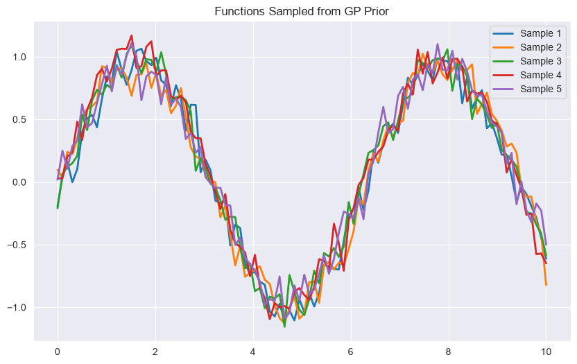
# Sample functions from GP prior
X_sample = np.linspace(0, 10, 100).reshape(-1, 1)
y_samples = gp.sample_y(X_sample, n_samples=5)
plt.figure(figsize=(10, 6))
for i in range(5):
plt.plot(X_sample, y_samples[:, i], lw=2, label=f'Sample {i+1}')
plt.title('Functions Sampled from GP Prior')
plt.legend()
plt.show()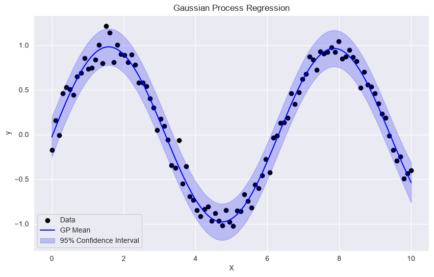
Dimensionality Reduction
Educational Objectives
Understand the curse of dimensionality
Explain the manifold hypothesis
Implement Principal Component Analysis (PCA)
Understand Kernel PCA for non-linear extensions
Apply manifold learning techniques (MDS, LLE, Isomap, t-SNE)
Key Concepts
Curse of Dimensionality
Manifold Hypothesis
Principal Component Analysis (PCA)
PCA finds orthogonal directions (principal components) that maximize variance. Steps:
Center the data:
Compute covariance matrix:
Eigendecomposition:
Select top eigenvectors
Practical Example: PCA for Visualization
import pandas as pd
from sklearn.decomposition import PCA
from sklearn.preprocessing import StandardScaler

# Load and clean data
df = pd.read_csv('machine-learning/DiabetesDataset.csv')
X = df.drop('Diabetes', axis=1)
y = df['Diabetes']

# Standardize data
scaler = StandardScaler()
X_scaled = scaler.fit_transform(X)

# Apply PCA
pca = PCA(n_components=2)
X_pca = pca.fit_transform(X_scaled)

# Plot
plt.figure(figsize=(10, 8))
plt.scatter(X_pca[:, 0], X_pca[:, 1], c=y, cmap='viridis', alpha=0.6)
plt.colorbar(label='Class')
plt.xlabel('Principal Component 1')
plt.ylabel('Principal Component 2')
plt.title('PCA: 2D Visualization')
plt.show()

# Explained variance
print(f"Explained variance ratio: {pca.explained_variance_ratio_}")
print(f"Total explained variance: {sum(pca.explained_variance_ratio_):.4f}")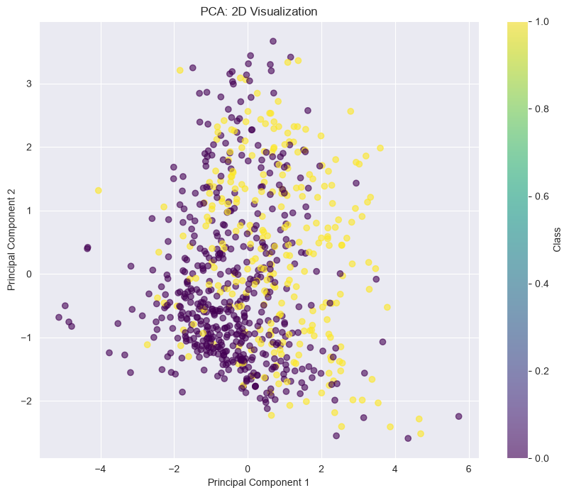
Explained variance ratio: [0.26179749 0.21640127]
Total explained variance: 0.4782
Kernel PCA
from sklearn.decomposition import KernelPCA

# Kernel PCA with RBF kernel
kpca = KernelPCA(n_components=2, kernel='rbf', gamma=0.04, fit_inverse_transform=True)
X_kpca = kpca.fit_transform(X_scaled)

# Plot
plt.figure(figsize=(10, 8))
plt.scatter(X_kpca[:, 0], X_kpca[:, 1], c=y, cmap='viridis', alpha=0.6)
plt.colorbar(label='Class')
plt.xlabel('Kernel PC 1')
plt.ylabel('Kernel PC 2')
plt.title('Kernel PCA: 2D Visualization')
plt.show()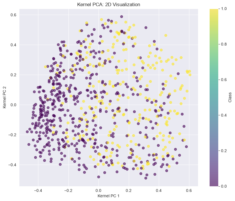
Manifold Learning Techniques
Preserves pairwise distances
Linear technique
Good for visualization
Preserves local structure
Non-linear technique
Excellent for visualization
Computationally expensive
Preserves local linear relationships
Non-linear technique
Good for manifold learning
Preserves geodesic distances
Non-linear technique
Uses neighborhood graph
from sklearn.manifold import TSNE

# t-SNE
tsne = TSNE(n_components=2, perplexity=30, random_state=42)
X_tsne = tsne.fit_transform(X_scaled[:1000])  # Use subset for speed

plt.figure(figsize=(10, 8))
plt.scatter(X_tsne[:, 0], X_tsne[:, 1], c=y[:1000], cmap='viridis', alpha=0.6)
plt.colorbar(label='Class')
plt.title('t-SNE: 2D Visualization')
plt.show()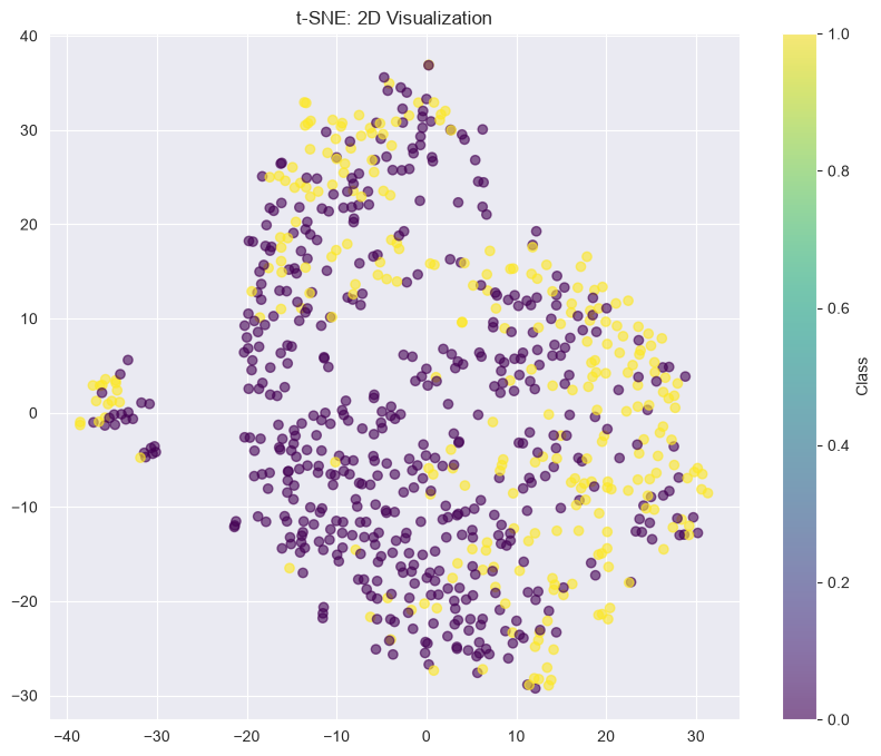
Cluster Analysis
Educational Objectives
Understand different clustering paradigms
Implement and interpret hierarchical clustering
Use the elbow method to determine optimal number of clusters
Apply partitioning methods like k-Means
Understand density-based clustering (DBSCAN)
Evaluate clustering results
Key Concepts
Types of Clustering
k-Means: Partitions data into k clusters
k-Medoids: Uses actual data points as centers
Fuzzy c-Means: Soft clustering (probabilistic)
Agglomerative: Bottom-up
Divisive: Top-down
Dendrogram: Visual representation
DBSCAN: Density-based spatial clustering
OPTICS: Similar to DBSCAN but more robust
HDBSCAN: Hierarchical DBSCAN
k-Means Algorithm
Initialize k cluster centers randomly
Assign each point to nearest cluster center
Recalculate cluster centers as mean of assigned points
Repeat steps 2-3 until convergence
Practical Example: k-Means Clustering
from sklearn.cluster import KMeans
from sklearn.metrics import silhouette_score, davies_bouldin_score
from sklearn.datasets import make_blobs
X, y = make_blobs(n_samples=300, centers=4, cluster_std=1.0, random_state=42)
# k-Means clustering
kmeans = KMeans(n_clusters=3, init='k-means++', max_iter=300, n_init=10, random_state=42)
clusters = kmeans.fit_predict(X)
# Plot clusters
plt.figure(figsize=(10, 8))
plt.scatter(X[:, 0], X[:, 1], c=clusters, cmap='viridis', alpha=0.6)
plt.scatter(kmeans.cluster_centers_[:, 0], kmeans.cluster_centers_[:, 1], s=200, c='red', marker='X', label='Centroids')
plt.legend()
plt.title('k-Means Clustering')
plt.show()
# Evaluate clustering
print(f"Silhouette Score: {silhouette_score(X, clusters):.4f}")
print(f"Davies-Bouldin Score: {davies_bouldin_score(X, clusters):.4f}")
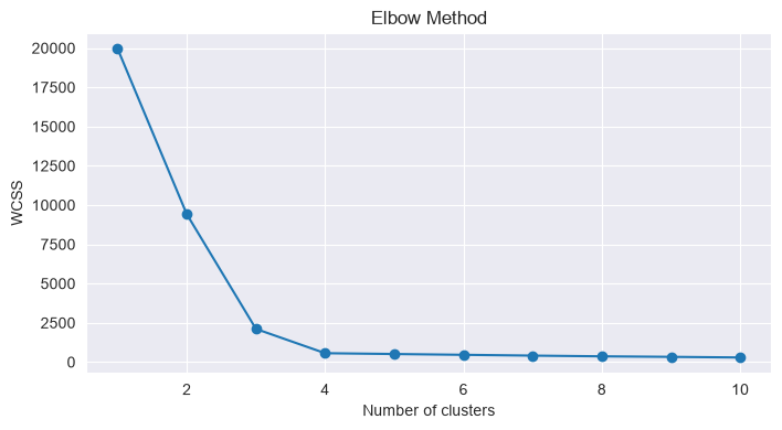
# Elbow method
wcss = []
for k in range(1, 11):
kmeans = KMeans(n_clusters=k, init='k-means++', random_state=42)
kmeans.fit(X)
wcss.append(kmeans.inertia_)
plt.figure(figsize=(8, 4))
plt.plot(range(1, 11), wcss, marker='o')
plt.xlabel('Number of clusters')
plt.ylabel('WCSS')
plt.title('Elbow Method')
plt.show()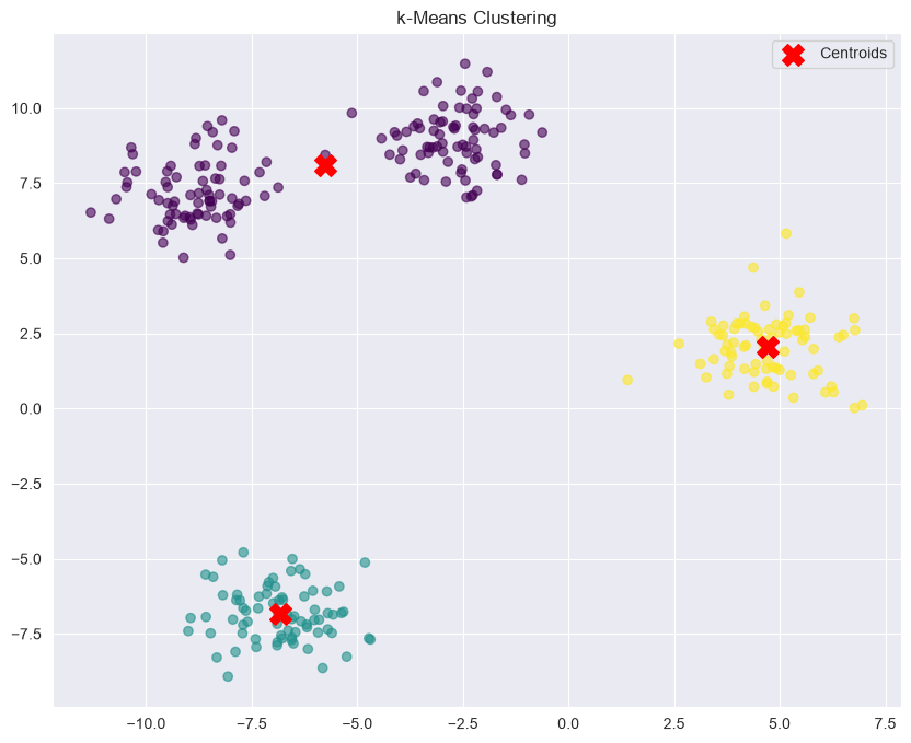
Silhouette Score: 0.7569
Davies-Bouldin Score: 0.3560
Hierarchical Clustering Example
from scipy.cluster.hierarchy import dendrogram, linkage, fcluster
from sklearn.datasets import make_blobs

X, y = make_blobs(n_samples=300, centers=4, cluster_std=1.0, random_state=42)

# Perform hierarchical clustering
Z = linkage(X, method='ward')

# Plot dendrogram
plt.figure(figsize=(12, 6))
dendrogram(Z, truncate_mode='level', p=12)
plt.title('Hierarchical Clustering Dendrogram')
plt.xlabel('Sample Index')
plt.ylabel('Distance')
plt.show()

# Cut dendrogram
clusters = fcluster(Z, t=10, criterion='distance')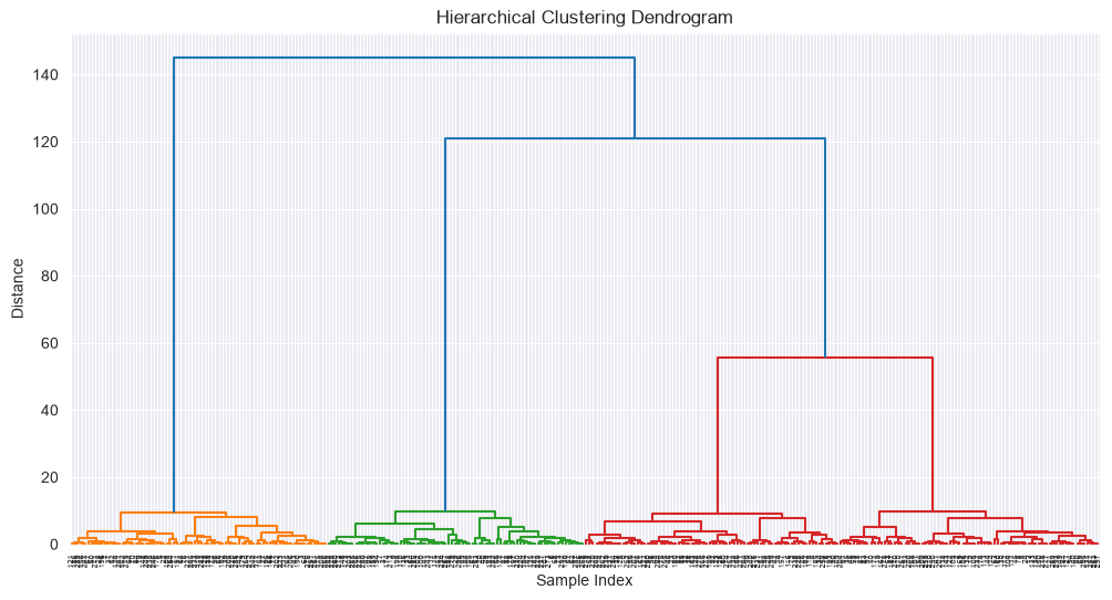
DBSCAN Example
from sklearn.cluster import DBSCAN
from sklearn.datasets import make_moons

X, y = make_moons(n_samples=300, noise=0.05, random_state=42)

# DBSCAN
dbscan = DBSCAN(eps=0.25, min_samples=5, metric='euclidean')
clusters = dbscan.fit_predict(X)

# Plot
plt.figure(figsize=(10, 8))
plt.scatter(X[:, 0], X[:, 1], c=clusters, cmap='viridis', alpha=0.6)
plt.title('DBSCAN Clustering')
plt.show()

# Count clusters and noise
n_clusters = len(set(clusters)) - (1 if -1 in clusters else 0)
n_noise = list(clusters).count(-1)
print(f"Number of clusters: {n_clusters}")
print(f"Number of noise points: {n_noise}")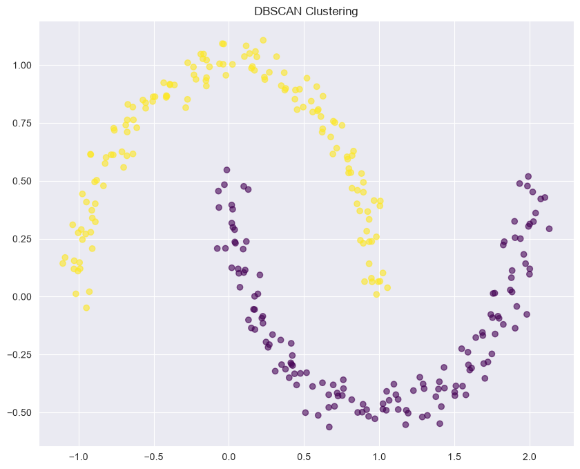
Number of clusters: 2
Number of noise points: 0
Gaussian Mixture Models & Expectation-Maximization
Educational Objectives
Understand Gaussian Mixture Models (GMMs)
Implement the Expectation-Maximization (EM) algorithm
Understand soft clustering vs. hard clustering
Apply GMMs to real-world data
Understand the relationship between GMMs and k-Means
Key Concepts
Gaussian Mixture Model
A probabilistic model that assumes data is generated from a mixture of several Gaussian distributions:
Where:
= Mixing coefficient,
= Mean of component k
= Covariance matrix of component k
Expectation-Maximization (EM) Algorithm
E-step (Expectation): Compute posterior probabilities (responsibilities)
M-step (Maximization): Update parameters using current responsibilities
Repeat until convergence
GMM vs. k-Means
| Aspect | GMM | k-Means |
|---|---|---|
| Clustering | Soft (probabilistic) | Hard (deterministic) |
| Cluster Shape | Elliptical | Spherical |
| Covariance | Can be different | Same (identity) |
| Probabilistic | Yes | No |
Practical Example: GMM with scikit-learn
from sklearn.mixture import GaussianMixture
from sklearn.datasets import make_blobs
X, y = make_blobs(n_samples=300, centers=4, cluster_std=1.0, random_state=42)
# Fit GMM
n_components = 2
gmm = GaussianMixture(n_components=n_components, covariance_type='full', random_state=42)
gmm.fit(X)
# Predict cluster assignments (hard clustering)
clusters = gmm.predict(X)
# Get probabilities (soft clustering)
probabilities = gmm.predict_proba(X)
# Plot clusters with uncertainty
plt.figure(figsize=(10, 8))
scatter = plt.scatter(X[:, 0], X[:, 1], c=clusters, cmap='viridis', alpha=0.6)
plt.title('GMM Clustering')
plt.colorbar(scatter, label='Cluster')
plt.show()
# Print model parameters
print(f"Means:\n{gmm.means_}")
print(f"Covariances:\n{gmm.covariances_}")
print(f"Weights:\n{gmm.weights_}")
# Calculate AIC and BIC
aic = gmm.aic(X)
bic = gmm.bic(X)
print(f"AIC: {aic}, BIC: {bic}")
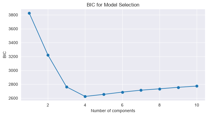
# Find optimal number of components using BIC
n_components_range = range(1, 11)
bic_scores = []
for n in n_components_range:
gmm = GaussianMixture(n_components=n, random_state=42)
gmm.fit(X)
bic_scores.append(gmm.bic(X))
plt.figure(figsize=(8, 4))
plt.plot(n_components_range, bic_scores, marker='o')
plt.xlabel('Number of components')
plt.ylabel('BIC')
plt.title('BIC for Model Selection')
plt.show()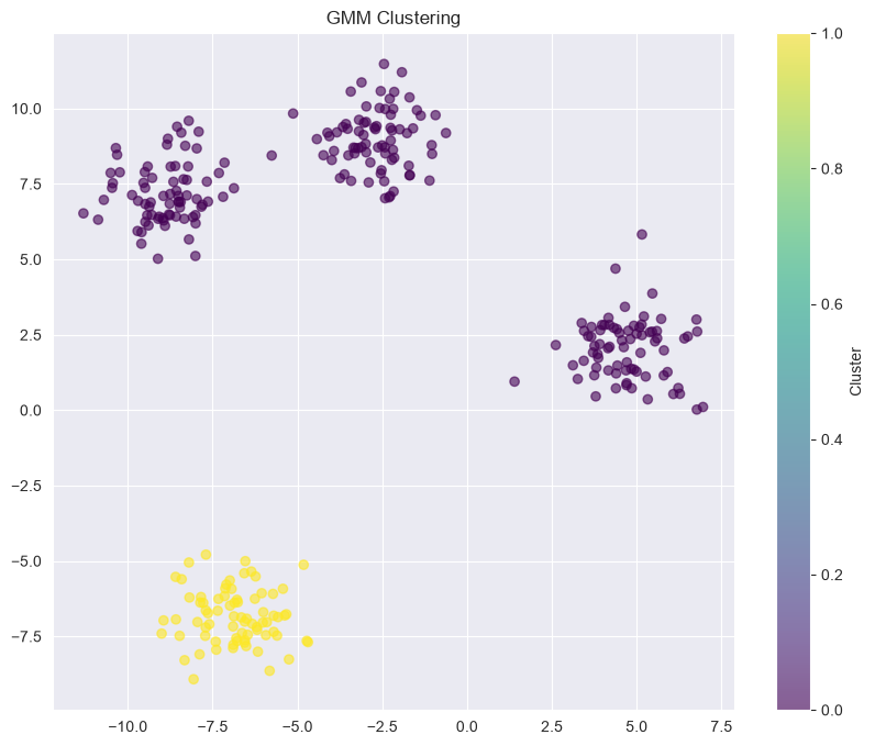
Means:
[[-2.26099844  6.07059032]
 [-6.83235214 -6.83045757]]
Covariances:
[[[ 31.61453403 -12.1886063 ]
  [-12.1886063    9.63288295]]

 [[  1.011053    -0.06122604]
  [ -0.06122604   0.79622858]]]
Weights:
[0.75000001 0.24999999]
AIC: 3181.6956036449124, BIC: 3222.4372108661305
Reinforcement Learning
Educational Objectives
Define finite Markov Decision Process (MDP) and Markov Reward Process (MRP)
Understand value iteration and Q-learning algorithms
Explain the difference between on-policy and off-policy learning
Explain the difference between value iteration and policy iteration
Understand the trade-off between exploitation and exploration
Key Concepts
Markov Decision Process (MDP)
A framework for modeling decision-making situations:
Where:
= Set of states
= Set of actions
= Transition probability
= Reward function
= Discount factor ()
Markov Property
Value Functions
Bellman Equation
Optimal Policy
Dynamic Programming Methods
Value Iteration
Policy Iteration
Policy Evaluation: Compute for current policy
Policy Improvement: Update policy to be greedy with respect to
Temporal Difference Learning
Q-Learning
Exploration vs. Exploitation
Try different actions to discover better strategies
Needed to find optimal policy
Can lead to suboptimal short-term rewards
Use known best action to maximize immediate reward
Can miss better long-term strategies
Suboptimal in the long run if overused
Common exploration strategies:
ε-greedy: Choose random action with probability ε
Decaying ε-greedy: ε decreases over time
Upper Confidence Bound (UCB): Balance exploration and exploitation
Thompson Sampling: Probabilistic approach based on uncertainty
On-Policy vs. Off-Policy
| Aspect | On-Policy | Off-Policy |
|---|---|---|
| Definition | Learns about and improves the same policy | Learns about one policy while following another |
| Example | SARSA | Q-Learning |
| Advantage | Directly learns the policy being followed | Can learn optimal policy while following exploratory policy |
| Disadvantage | Must balance exploration/exploitation | More complex, can be unstable |
Practical Example: Q-Learning for Frozen Lake
import gym
import numpy as np
np.bool8 = np.bool # Fix for AttributeError: module 'numpy' has no attribute 'bool8'

# Create FrozenLake environment
env = gym.make('FrozenLake-v1', is_slippery=False)

# Initialize Q-table
Q = np.zeros((env.observation_space.n, env.action_space.n))

# Hyperparameters
alpha = 0.8  # Learning rate
gamma = 0.95  # Discount factor
epsilon = 0.1  # Exploration rate
episodes = 10000

# Q-learning algorithm
for episode in range(episodes):
    state = env.reset()[0]
    done = False
    truncated = False

    while not done and not truncated:
        # Epsilon-greedy action selection
        if np.random.uniform(0, 1) < epsilon:
            action = env.action_space.sample()  # Explore
        else:
            action = np.argmax(Q[state, :])  # Exploit

        # Take action
        next_state, reward, done, truncated, info = env.step(action)

        # Q-learning update
        best_next_action = np.argmax(Q[next_state, :])
        td_target = reward + gamma * Q[next_state, best_next_action]
        td_error = td_target - Q[state, action]
        Q[state, action] += alpha * td_error

        # Update state
        state = next_state

# Test the learned policy
state = env.reset()[0]
done = False
truncated = False

while not done and not truncated:
    action = np.argmax(Q[state, :])
    state, reward, done, truncated, info = env.step(action)
    if done or truncated:
        print(f"Final reward: {reward}")
        break
env.close()
Final reward: 0.0
Ensemble Methods
Educational Objectives
Understand ensemble learning principles
Implement bagging methods (e.g., Random Forest)
Implement boosting methods (e.g., AdaBoost, Gradient Boosting)
Understand the bias-variance tradeoff in ensemble methods
Apply ensemble methods to real-world problems
Key Concepts
Ensemble Learning
Combining multiple models to improve performance:
Types of Ensembles
Principle: Reduce variance by averaging multiple models
Method: Train models on different bootstrap samples
Example: Random Forest
Effect: Reduces variance, prevents overfitting
Principle: Reduce bias by sequentially correcting errors
Method: Train models sequentially, each focusing on previous errors
Examples: AdaBoost, Gradient Boosting, XGBoost
Effect: Reduces bias, improves accuracy
Gini Impurity
Gini Impurity is a measure of node purity used in decision trees (CART algorithm). It quantifies the probability of misclassifying a randomly selected sample in a node if it were labeled according to the distribution of classes in the node.
For a node with classes, where is the proportion of class :
Range: 0 (perfectly pure) to (maximally impure)
Interpretation: Lower values indicate higher purity
def gini_impurity(counts):
    total = sum(counts)

    if total == 0:
        return 0.0

    probabilities = [c / total for c in counts]
    return 1 - sum(p**2 for p in probabilities)


def gini_split(*children):
    """
    Compute the weighted Gini impurity of an arbitrary split.

    Parameters
    ----------
    *children : iterable of class counts
        Examples:
            [7, 0]
            [10, 4]
            [3, 2, 5]   # multiclass

    Returns
    -------
    float
        Weighted Gini impurity of the split.
    """
    total_samples = sum(sum(child) for child in children)

    if total_samples == 0:
        return 0.0

    return sum(
        (sum(child) / total_samples) * gini_impurity(child)
        for child in children
    )

print(gini_split([7, 0], [9, 4]))
0.276923076923077
Random Forest
An ensemble of decision trees trained on bootstrap samples with feature subsampling:
Create bootstrap samples (with replacement)
For each sample, train a decision tree on a random subset of features
Average predictions from all trees
Boosting Methods
Idea: Give more weight to misclassified samples
Algorithm: Sequentially train models, reweighting data
Weight Update: Increase weights for misclassified samples
Idea: Fit new models to residual errors
Algorithm: Each new model corrects errors of previous ensemble
Loss: Minimizes loss function (e.g., MSE, log-loss)
Practical Example: Random Forest
import seaborn as sns
from sklearn.ensemble import RandomForestClassifier
from sklearn.metrics import accuracy_score
from sklearn.model_selection import train_test_split
# Load and clean data
df = pd.read_csv('machine-learning/DiabetesDataset.csv')
X = df.drop('Diabetes', axis=1)
y = df['Diabetes']
X_train, X_test, y_train, y_test = train_test_split(X, y, test_size=0.2, random_state=42)
# Random Forest
rf = RandomForestClassifier(
n_estimators=100,
max_depth=None,
min_samples_split=2,
min_samples_leaf=1,
max_features='sqrt',
bootstrap=True,
random_state=42
)
rf.fit(X_train, y_train)
y_pred_rf = rf.predict(X_test)
print(f"Random Forest Accuracy: {accuracy_score(y_test, y_pred_rf):.4f}")
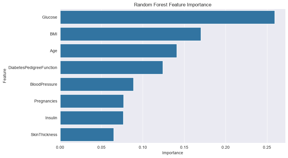
# Feature importance
importances = rf.feature_importances_
feature_importance = pd.DataFrame({'Feature': X.columns, 'Importance': importances}).sort_values('Importance', ascending=False)
plt.figure(figsize=(10, 6))
sns.barplot(x='Importance', y='Feature', data=feature_importance)
plt.title('Random Forest Feature Importance')
plt.show()Random Forest Accuracy: 0.7208
Gradient Boosting Example
from sklearn.ensemble import GradientBoostingClassifier
# Gradient Boosting
gb = GradientBoostingClassifier(
n_estimators=100,
learning_rate=0.1,
max_depth=3,
min_samples_split=2,
min_samples_leaf=1,
random_state=42
)
gb.fit(X_train, y_train)
y_pred_gb = gb.predict(X_test)
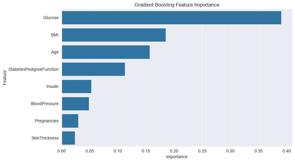
print(f"Gradient Boosting Accuracy: {accuracy_score(y_test, y_pred_gb):.4f}")
# Plot feature importance
feature_importance_gb = pd.DataFrame({'Feature': X.columns, 'Importance': gb.feature_importances_}).sort_values('Importance', ascending=False)
plt.figure(figsize=(10, 6))
sns.barplot(x='Importance', y='Feature', data=feature_importance_gb)
plt.title('Gradient Boosting Feature Importance')
plt.show()Gradient Boosting Accuracy: 0.7468
AdaBoost Example
from sklearn.ensemble import AdaBoostClassifier

ada = AdaBoostClassifier(n_estimators=100, learning_rate=1.0, random_state=42)
ada.fit(X_train, y_train)
y_pred_ada = ada.predict(X_test)
print(f"AdaBoost Accuracy: {accuracy_score(y_test, y_pred_ada):.4f}")
AdaBoost Accuracy: 0.7403
Generative AI and Wrap-Up
Educational Objectives
Understand the landscape of generative AI
Explain different generative modeling approaches
Understand applications and limitations of generative models
Reflect on the future of machine learning
Integrate knowledge from all course topics
Key Concepts
Generative AI Overview
Generative AI models learn to generate new data that resembles the training data:
Idea: Two neural networks compete (generator vs. discriminator)
Training: Generator tries to fool discriminator
Applications: Image generation, style transfer
Idea: Learn probability distribution of data
Training: Maximize likelihood of data
Applications: Image generation, anomaly detection
Idea: Predict next token in sequence
Training: Self-supervised on vast text data
Applications: Text generation, translation, coding
Generative Model Types
| Model | Approach | Training | Applications |
|---|---|---|---|
| GAN | Adversarial | Minimax game | Images, audio |
| VAE | Probabilistic | Maximum likelihood | Images, data generation |
| Autoregressive | Sequential | Next token prediction | Text, audio, video |
| Diffusion | Iterative denoising | Noise removal | Images, audio |
Trends
Scale: Models continue to grow in size and capability
Efficiency: More efficient architectures and training methods
Multimodality: Models that understand multiple data types
Alignment: Ensuring models behave as intended (safety, ethics)
Interpretability: Understanding model decisions
Automation: AutoML and hyperparameter optimization