Predictive Modeling
Exam Strategies & Common Pitfalls
Common Pitfalls to Avoid
Linear Regression:
✗ Confusing prediction interval with confidence interval
✗ Using to compare models with different sample sizes
✗ Ignoring collinearity when standard errors are large
✗ Including interaction without main effects
✗ Forgetting to check residual plots
Logistic Regression:
✗ Interpreting as change in probability (it’s log-odds!)
✗ Confusing odds with probability
✗ Trusting high accuracy with class imbalance
✗ Using wrong metrics (accuracy vs F1/recall/precision)
Model Selection:
✗ Using forward selection as if it’s optimal (it’s greedy!)
✗ Confusing minimizing AIC with maximizing (BIC same)
✗ Forgetting to standardize before ridge/lasso
Time Series:
✗ Fitting ARMA to non-stationary series (must difference first!)
✗ Assuming MA implies non-stationary (MA is always stationary)
✗ Confusing ACF cutoff (MA) with PACF cutoff (AR)
✗ Not checking if roots satisfy stationarity condition
✗ Forgetting that forecasts converge to mean (long-term)
Hypothesis Testing:
✗ Confusing failing to reject with accepting
✗ Using t-test when F-test is needed (multiple coefficients)
✗ Not reporting degrees of freedom for test statistics
✗ Misinterpreting p-value as probability is true
Calculations:
✗ Arithmetic errors (double-check!)
✗ Wrong degrees of freedom ( vs vs )
✗ Forgetting square root in RMSE or SE formulas
✗ Sign errors (especially with differencing)
Key Concepts Summary
When to Use Each Method:
| Goal | Method |
|---|---|
| Quantitative , linear relationship | Linear regression |
| Binary | Logistic regression |
| Non-linear relationship | Polynomial regression, transformation |
| Variable selection | Stepwise, lasso |
| Multicollinearity | Ridge regression, VIF check |
| Time series, stationary | ARMA |
| Time series, trend | ARIMA (difference first) |
| Time series, seasonality | SARIMA, STL decomposition |
| Model comparison | AIC, BIC, CV, adj- |
| Check assumptions | Residual plots, diagnostic tests |
Stationarity?
Plot series, check ACF
If trend/changing variance → transform or difference
If seasonal → seasonal differencing or STL
AR vs MA vs ARMA?
ACF cuts off, PACF tails → MA()
PACF cuts off, ACF tails → AR()
Both tail off → ARMA()
Which regularization?
Want variable selection → Lasso
Many correlated predictors, all important → Ridge
Not sure → Try both, compare CV error
Which interval?
Predict mean/average → Confidence interval
Predict single observation → Prediction interval
Key Things to Remember
increases with more predictors, use adj-
F-test for overall significance, t-test for individual coefficients
VIF suggests collinearity
Cook’s suggests influential point
Logistic: coefficients are log-odds, not probabilities
MA is always stationary, AR requires roots
ACF for MA, PACF for AR
Difference before fitting ARIMA to non-stationary series
Always standardize before ridge/lasso
F1 score for imbalanced classification
Essential Formulas & Key Calculations
Regression Formulas
:
Adjusted :
F-statistic:
Confidence interval for :
VIF:
Saturated Model
Problem: observations, parameters
Perfect fit: , all residuals
Estimate of
Interpretation: Complete overfitting, no generalization
Logistic Regression Calculations
From to probability:
Linear predictor:
Probability:
Odds:
Log-odds:
From probability to odds:
Example: (or 1:4)
Example: (or 4:1)
From odds to probability:
Example:
Log-odds (logit):
Example:
AR Process Variance
AR(1): ,
Take variance:
Solve:
Stationary mean:
Take expectation:
Solve:
Characteristic Polynomial Check
AR(2) Example:
Characteristic polynomial:
Solve for roots:
Check: If both → stationary
Alternative: Rewrite as polynomial in and check roots inside unit circle
MA(1) Autocovariance
Model:
Variance:
Lag-1 Covariance:
Lag- Covariance (): (no overlapping terms)
ACF:
for
# Compute Autocovariance+Autocorrelation at Lags 0-N:
from statsmodels.tsa.arima_process import ArmaProcess

ar_params = [1, -0.5, -1/3]  # 1 - 0.5L - (1/3)L^2
ma_params = [1]  # no MA terms
process = ArmaProcess(ar_params, ma_params)

# Autocovariance+Autocorrelation at lags 0 through n
var_X = process.acovf()[0] # variance at lag 0 (σ²_X)
acov = process.acovf()
for k, acov_at_lag_k in enumerate(acov):
    acorr_at_lag_k = acov_at_lag_k / var_X
    print(f"γ({k}) = {acov_at_lag_k:.6f}, γ({k})/σ²_X = {acorr_at_lag_k:.6f}")
    if (acorr_at_lag_k) < 0.1: break
γ(0) = 2.571429, γ(0)/σ²_X = 1.000000
γ(1) = 1.928571, γ(1)/σ²_X = 0.750000
γ(2) = 1.821429, γ(2)/σ²_X = 0.708333
γ(3) = 1.553571, γ(3)/σ²_X = 0.604167
γ(4) = 1.383929, γ(4)/σ²_X = 0.538194
γ(5) = 1.209821, γ(5)/σ²_X = 0.470486
γ(6) = 1.066220, γ(6)/σ²_X = 0.414641
γ(7) = 0.936384, γ(7)/σ²_X = 0.364149
γ(8) = 0.823599, γ(8)/σ²_X = 0.320288
γ(9) = 0.723927, γ(9)/σ²_X = 0.281527
γ(10) = 0.636497, γ(10)/σ²_X = 0.247526
γ(11) = 0.559557, γ(11)/σ²_X = 0.217606
γ(12) = 0.491944, γ(12)/σ²_X = 0.191312
γ(13) = 0.432491, γ(13)/σ²_X = 0.168191
γ(14) = 0.380227, γ(14)/σ²_X = 0.147866
γ(15) = 0.334277, γ(15)/σ²_X = 0.129997
γ(16) = 0.293881, γ(16)/σ²_X = 0.114287
γ(17) = 0.258366, γ(17)/σ²_X = 0.100476
γ(18) = 0.227143, γ(18)/σ²_X = 0.088334
Linear Regression Fundamentals
Model Assumptions
The linear regression model assumes:
Linearity:
Independence: errors are independent
Homoscedasticity: (constant variance)
Normality: (needed for inference)
Check via residual plots!
Simple Linear Regression
import numpy as np
import pandas as pd
import statsmodels.api as sm
from TMA_def import model_plot

np.random.seed(0)

n = 100
X = np.linspace(0, 10, n)
Y = 2 + 3 * X + np.random.normal(scale=2.0, size=n)

df = pd.DataFrame({"X": X, "Y": Y})

X_sm = sm.add_constant(df["X"])  # adds a column named "const"
model = sm.OLS(df["Y"], X_sm).fit()

model_plot(df['X'], Y, model)
print(model.summary())

RES = model.resid             # residuals (vector)
TSS = model.centered_tss      # total sum of squares (around mean)
ESS = model.ess               # explained sum of squares
RSS = model.ssr               # residual sum of squares
R2  = model.rsquared          # R-squared
RSE = model.resid.std(ddof=model.df_model + 1)

print(f"TSS = {TSS:.3f}, ESS = {ESS:.3f}, RSS = {RSS:.3f}, R2 = {R2:.3f}, RSE = {RSE:.3f}")
OLS Regression Results
==============================================================================
Dep. Variable: Y R-squared: 0.948
Model: OLS Adj. R-squared: 0.947
Method: Least Squares F-statistic: 1786.
Date: Wed, 28 Jan 2026 Prob (F-statistic): 1.01e-64
Time: 19:11:29 Log-Likelihood: -211.62
No. Observations: 100 AIC: 427.2
Df Residuals: 98 BIC: 432.5
Df Model: 1
Covariance Type: nonrobust
==============================================================================
coef std err t P>|t| [0.025 0.975]
------------------------------------------------------------------------------
const 2.4169 0.403 6.002 0.000 1.618 3.216
X 2.9405 0.070 42.263 0.000 2.802 3.079
==============================================================================
Omnibus: 0.397 Durbin-Watson: 1.841
Prob(Omnibus): 0.820 Jarque-Bera (JB): 0.556
Skew: -0.036 Prob(JB): 0.757
Kurtosis: 2.642 Cond. No. 11.7
==============================================================================
Notes:
[1] Standard Errors assume that the covariance matrix of the errors is correctly specified.
TSS = 7754.512, ESS = 7351.188, RSS = 403.324, R2 = 0.948, RSE = 2.029
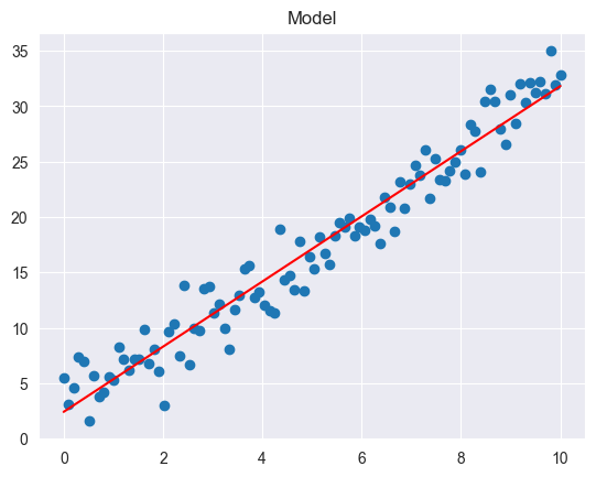
Model:
: intercept (value of when )
: slope (change in for unit change in )
: error term with ,
Least Squares Estimation: Minimize to find and
Key Quantities:
TSS (Total Sum of Squares) (total variance in )
RSS (Residual Sum of Squares) (unexplained variance)
(fraction of variance explained, )
RSE (residual standard error, estimate of )
Multiple Linear Regression
import numpy as np
import pandas as pd
import statsmodels.api as sm

# Example multiple linear regression with two predictors
np.random.seed(1)

n = 100
X1 = np.random.normal(size=n)
X2 = np.random.normal(size=n)

# True model: Y = 1 + 2*X1 - 1*X2 + noise
Y = 1 + 2 * X1 - 1 * X2 + np.random.normal(scale=1.0, size=n)

df = pd.DataFrame({"X1": X1, "X2": X2, "Y": Y})

X_sm = sm.add_constant(df[["X1", "X2"]])
model = sm.OLS(df["Y"], X_sm).fit()

print(model.summary())
OLS Regression Results
==============================================================================
Dep. Variable: Y R-squared: 0.770
Model: OLS Adj. R-squared: 0.766
Method: Least Squares F-statistic: 162.8
Date: Wed, 28 Jan 2026 Prob (F-statistic): 1.01e-31
Time: 19:11:29 Log-Likelihood: -140.24
No. Observations: 100 AIC: 286.5
Df Residuals: 97 BIC: 294.3
Df Model: 2
Covariance Type: nonrobust
==============================================================================
coef std err t P>|t| [0.025 0.975]
------------------------------------------------------------------------------
const 0.9802 0.101 9.672 0.000 0.779 1.181
X1 1.9381 0.113 17.107 0.000 1.713 2.163
X2 -0.7816 0.108 -7.264 0.000 -0.995 -0.568
==============================================================================
Omnibus: 0.256 Durbin-Watson: 2.195
Prob(Omnibus): 0.880 Jarque-Bera (JB): 0.076
Skew: -0.063 Prob(JB): 0.963
Kurtosis: 3.048 Cond. No. 1.24
==============================================================================
Notes:
[1] Standard Errors assume that the covariance matrix of the errors is correctly specified.
Model:
Hypothesis Testing:
Individual t-test: Test vs
Test statistic:
Reject if or if p-value
if is less than (i.e. 0.05): The parameter is significant, reject
else if is greater than or equal (i.e. 0.05): Parameter not significant, retain
from scipy.stats import t

# the 97.5% quantile of a t-distribution with 18 degrees of freedom
t.ppf(0.975, df=18)2.10092204024096Global F-test: Test (no predictors useful)
If true, expect
If true (at least one ), expect
Large and small p-value → reject
Partial F-test: Test if subset of coefficients are zero
X_reduced = sm.add_constant(df[["X1"]])
model_reduced = sm.OLS(df["Y"], X_reduced).fit()

# The output gives the F statistic, its p-value,
# and the degrees of freedom difference between models:
f_stat, p_value, df_diff = model.compare_f_test(model_reduced)
f_stat, p_value, df_diff
(52.76773415397895, 9.481480727697889e-11, 1.0)( coefficients)
: smaller model (without predictors)
RSS: larger model (with all predictors)
Important Insight: If all individual t-tests fail to reject but global F-test is significant → collinearity problem!
Confidence vs. Prediction Intervals
import numpy as np
import pandas as pd
import statsmodels.api as sm

np.random.seed(0)

n = 100
X = np.linspace(0, 10, n)
Y = 2 + 3 * X + np.random.normal(scale=2.0, size=n)

df = pd.DataFrame({"X": X, "Y": Y})

X_sm = sm.add_constant(df["X"])  # adds a column named "const"

model = sm.OLS(df["Y"], X_sm).fit()

# Predict at new point(s):
x0 = [5.0, 7.0]
x0_sm = sm.add_constant(x0, has_constant="add")
pred = model.get_prediction(x0_sm)

print("\nPrediction Summary (Intervals = 5%):\n", pred.summary_frame(alpha=0.05)) # 95% intervals
# mean                           := predicted response
# mean_se                        := predicted standard error
# [mean_ci_lower, mean_ci_upper] := confidence interval
# [obs_ci_lower, obs_ci_upper]   := prediction interval

print("\nConfidence Interval 5%:\n", pred.conf_int(alpha=0.05))
Prediction Summary (Intervals = 5%):
         mean   mean_se  mean_ci_lower  mean_ci_upper  obs_ci_lower  \
0  17.119616  0.202868      16.717031      17.522202     13.073682
1  23.000685  0.246006      22.512494      23.488876     18.945338

   obs_ci_upper
0     21.165551
1     27.056033

Confidence Interval 5%:
 [[16.7170305  17.52220156]
 [22.51249409 23.48887648]]
Confidence Interval: For mean response
Estimates average for given
Formula:
Narrower interval
Prediction Interval: For individual response
Predicts single observation for given
Formula:
Wider interval (includes both model uncertainty and )
Which to use?
Mayor wants prognosis for his town → Prediction interval (single observation)
Researcher wants average effect → Confidence interval (mean)
import numpy as np
import pandas as pd
import statsmodels.api as sm
from TMA_def import tma_plots

np.random.seed(0)

n = 100
X = np.linspace(0, 10, n)
Y = 2 + 3 * X + np.random.normal(scale=2.0, size=n)

df = pd.DataFrame({"X": X, "Y": Y})

X_sm = sm.add_constant(df["X"])  # adds a column named "const"

model = sm.OLS(df["Y"], X_sm).fit()

tma_plots(model)
Tukey-Anscombe Plot (Residuals vs Fitted Values):
import numpy as np
import pandas as pd
import statsmodels.api as sm
import matplotlib.pyplot as plt
from TMA_def import plot_residuals

np.random.seed(0)

n = 100
X = np.linspace(0, 10, n)
Y = 2 + 3 * X + np.random.normal(scale=2.0, size=n)

df = pd.DataFrame({"X": X, "Y": Y})

X_sm = sm.add_constant(df["X"])  # adds a column named "const"

model = sm.OLS(df["Y"], X_sm).fit()

fig = plt.figure(figsize = (4, 4))
ax = fig.add_subplot(1, 1, 1)
plot_residuals(ax, model.fittedvalues, model.resid, n_samp=1000, title='Tukey-Anscombe plot - Residuals vs Fitted')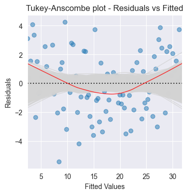
What to look for: Random scatter around zero
Patterns indicate problems:
Curve/non-linear pattern → non-linearity (try polynomial or transformation)
Funnel shape → heteroscedasticity
Outliers → investigate data quality
Scale-Location Plot ( vs fitted):
import numpy as np
import pandas as pd
import statsmodels.api as sm
import matplotlib.pyplot as plt
from TMA_def import plot_scale_loc

np.random.seed(0)

n = 100
X = np.linspace(0, 10, n)
Y = 2 + 3 * X + np.random.normal(scale=2.0, size=n)

df = pd.DataFrame({"X": X, "Y": Y})

X_sm = sm.add_constant(df["X"])  # adds a column named "const"

model = sm.OLS(df["Y"], X_sm).fit()

fig = plt.figure(figsize = (4, 4))
ax = fig.add_subplot(1, 1, 1)
plot_scale_loc(ax, model.fittedvalues, np.sqrt(np.abs(model.get_influence().resid_studentized_internal)), n_samp=1000, x_lab='Fitted values')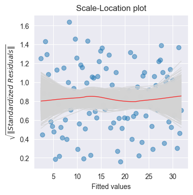
Purpose: Check homoscedasticity (constant variance)
Good: Horizontal line with random scatter
Bad: Increasing/decreasing trend → heteroscedasticity
Normal Q-Q Plot:
import numpy as np
import pandas as pd
import statsmodels.api as sm
import matplotlib.pyplot as plt
from TMA_def import plot_QQ

np.random.seed(0)

n = 100
X = np.linspace(0, 10, n)
Y = 2 + 3 * X + np.random.normal(scale=2.0, size=n)

df = pd.DataFrame({"X": X, "Y": Y})

X_sm = sm.add_constant(df["X"])  # adds a column named "const"

model = sm.OLS(df["Y"], X_sm).fit()

fig = plt.figure(figsize = (4, 4))
ax = fig.add_subplot(1, 1, 1)
plot_QQ(ax, model.get_influence().resid_studentized_internal, n_samp=1000, title='Normal plot or Q-Q plot')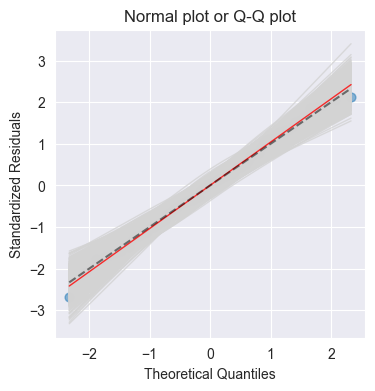
Purpose: Check normality of residuals
Good: Points follow diagonal line
Bad: Deviations at tails → heavy-tailed/skewed distribution
Residuals vs Leverage:
import numpy as np
import pandas as pd
import statsmodels.api as sm
import matplotlib.pyplot as plt
from TMA_def import plot_cooks

np.random.seed(0)

n = 100
X = np.linspace(0, 10, n)
Y = 2 + 3 * X + np.random.normal(scale=2.0, size=n)

df = pd.DataFrame({"X": X, "Y": Y})

X_sm = sm.add_constant(df["X"])  # adds a column named "const"

model = sm.OLS(df["Y"], X_sm).fit()

res_inf = model.get_influence() # Influence of the Residuals
res_standard = res_inf.resid_studentized_internal # Studentized residuals using variance from OLS
res_inf_leverage = res_inf.hat_matrix_diag
x_min, x_max = min(res_inf_leverage) - 0.005, max(res_inf_leverage) + 0.01
y_min, y_max = min(res_standard) - 1, max(res_standard) + 1

fig = plt.figure(figsize = (4, 4))
ax = fig.add_subplot(1, 1, 1)
plot_cooks(ax, res_inf_leverage, res_standard, n_pred=1, x_lim=[x_min, x_max], y_lim=[y_min, y_max])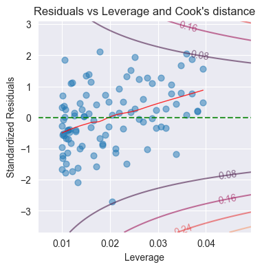
Purpose: Identify influential observations
Shows Cook’s distance contours
Points outside Cook’s or 1.0 are influential
Influential Points
Leverage ():
Measures how far predictor values are from
High leverage:
High leverage doesn’t mean influential!
Cook’s Distance ():
Measures influence of observation on fitted values
Combines leverage and residual size
Problematic: or
Influential points have high Cook’s
Standardized Residuals:
Outlier if: (or for stricter criterion)
Decision Tree:
High leverage + large residual → influential (investigate!)
High leverage + small residual → not influential (okay)
Low leverage + large residual → outlier but not influential
Low leverage + small residual → typical observation
import numpy as np
import pandas as pd
import statsmodels.api as sm
from statsmodels.stats.outliers_influence import variance_inflation_factor

np.random.seed(1)

n = 100
X1 = np.random.normal(size=n)
X2 = np.random.normal(size=n)
Y = 1 + 2 * X1 - 1 * X2 + np.random.normal(scale=1.0, size=n)
df = pd.DataFrame({"X1": X1, "X2": X2, "Y": Y})

X_vif = sm.add_constant(df[["X1", "X2"]])

vif_data = []
for j, col in enumerate(X_vif.columns):
    vif = variance_inflation_factor(X_vif.values, j)
    vif_data.append((col, vif))

vif_data
[('const', 1.0297726694375249),
('X1', 1.0082820653058149),
('X2', 1.0082820653058144)]from regression of on all other predictors
Interpretation:
: no collinearity
: moderate collinearity
: severe collinearity (problematic!)
Effects of Collinearity:
Inflates standard errors of coefficients
Makes coefficients unstable (sensitive to data changes)
Reduces statistical power (harder to reject )
Difficult to interpret individual coefficients
Does NOT reduce or predictive accuracy!
Solutions:
Remove correlated predictors
Combine correlated predictors (e.g., average)
Use ridge regression or lasso
Increase sample size
Variable transformation (e.g., center variables)
import numpy as np
import pandas as pd
import statsmodels.api as sm

np.random.seed(123)

# Create categorical predictor with 3 levels
n = 150
X = np.random.choice(["African American", "Asian", "Caucasian"], size=n, p=[0.4, 0.3, 0.3])

# True means: African American ~ 50, Asian ~ 55, Caucasian ~ 52 (all with sd 3)
means = { "African American": 50, "Asian": 55, "Caucasian": 52 }
Y = np.array([np.random.normal(loc=means[x], scale=3.0) for x in X])

df = pd.DataFrame({"ethnicity": X, "Y": Y})

# Automatically create k-1 dummies with get_dummies (drop_first=True)
X_dummy = pd.get_dummies(df["ethnicity"], drop_first=True, dtype=float)
X_dummy = sm.add_constant(X_dummy)
print(X_dummy.head())

model = sm.OLS(df["Y"], X_dummy).fit()
print(model.summary())
const Asian Caucasian
0 1.0 1.0 0.0
1 1.0 0.0 0.0
2 1.0 0.0 0.0
3 1.0 1.0 0.0
4 1.0 0.0 1.0
OLS Regression Results
==============================================================================
Dep. Variable: Y R-squared: 0.368
Model: OLS Adj. R-squared: 0.359
Method: Least Squares F-statistic: 42.77
Date: Wed, 28 Jan 2026 Prob (F-statistic): 2.29e-15
Time: 19:11:43 Log-Likelihood: -363.41
No. Observations: 150 AIC: 732.8
Df Residuals: 147 BIC: 741.9
Df Model: 2
Covariance Type: nonrobust
==============================================================================
coef std err t P>|t| [0.025 0.975]
------------------------------------------------------------------------------
const 50.3071 0.365 137.793 0.000 49.586 51.029
Asian 4.6013 0.521 8.832 0.000 3.572 5.631
Caucasian 0.8386 0.577 1.453 0.148 -0.302 1.979
==============================================================================
Omnibus: 5.616 Durbin-Watson: 1.800
Prob(Omnibus): 0.060 Jarque-Bera (JB): 7.720
Skew: -0.149 Prob(JB): 0.0211
Kurtosis: 4.071 Cond. No. 3.57
==============================================================================
Notes:
[1] Standard Errors assume that the covariance matrix of the errors is correctly specified.
Two Levels (e.g., Gender: Male/Female):
Create one dummy variable: if Female, if Male
Model:
Interpretation:
: mean for males (baseline)
: mean for females
: difference between females and males
Test tests if gender matters
Three Levels (e.g., Ethnicity: Asian, Caucasian, African American):
Create two dummy variables ( levels → dummies):
if Asian, 0 otherwise
if Caucasian, 0 otherwise
African American is baseline (both , )
Model:
Interpretation:
: mean for African Americans (baseline)
: mean for Asians
: mean for Caucasians
: difference between Asian and African American
: difference between Caucasian and African American
Key Rule: For categories, need dummy variables (one category is baseline)
Baseline Choice: Arbitrary, doesn’t affect model fit, only interpretation
Interaction Effects
Model with Interaction:
When : Effect of on depends on value of (synergy/interaction)
import numpy as np
import pandas as pd
import statsmodels.api as sm

np.random.seed(123)

n = 200
X1 = np.random.uniform(0, 10, size=n)
X2 = np.random.uniform(0, 5, size=n)

beta0_true = 1.0
beta1_true = 2.0
beta2_true = 1.0
beta3_true = 0.5

noise = np.random.normal(scale=2.0, size=n)
Y = beta0_true + beta1_true * X1 + beta2_true * X2 + beta3_true * X1 * X2 + noise

df = pd.DataFrame({"X1": X1, "X2": X2, "Y": Y})

# Y = beta0 + b1*X1 + b2*X2 + b3*X1*X2
X = sm.add_constant(df[["X1", "X2"]])
X["X1*X2"] = df["X1"] * df["X2"]

model = sm.OLS(df["Y"], X).fit()
print(model.summary())

# To assess significance of X1*X2 in the output:
# Because P>|t| = 0.000 (is less than 5%) and the
# CI [0.438, 0.585] does not contain 0, the interaction term
# is significant.
OLS Regression Results
==============================================================================
Dep. Variable: Y R-squared: 0.964
Model: OLS Adj. R-squared: 0.963
Method: Least Squares F-statistic: 1750.
Date: Wed, 28 Jan 2026 Prob (F-statistic): 3.46e-141
Time: 19:11:43 Log-Likelihood: -417.85
No. Observations: 200 AIC: 843.7
Df Residuals: 196 BIC: 856.9
Df Model: 3
Covariance Type: nonrobust
==============================================================================
coef std err t P>|t| [0.025 0.975]
------------------------------------------------------------------------------
const 0.7644 0.594 1.287 0.200 -0.407 1.936
X1 1.9915 0.101 19.673 0.000 1.792 2.191
X2 1.0108 0.216 4.676 0.000 0.584 1.437
X1*X2 0.5114 0.037 13.718 0.000 0.438 0.585
==============================================================================
Omnibus: 0.401 Durbin-Watson: 1.928
Prob(Omnibus): 0.818 Jarque-Bera (JB): 0.547
Skew: -0.067 Prob(JB): 0.761
Kurtosis: 2.781 Cond. No. 77.0
==============================================================================
Notes:
[1] Standard Errors assume that the covariance matrix of the errors is correctly specified.
Rewrite to see interaction:
Intercept for : (changes with )
Slope for : (changes with )
Example (Advertising):
: spending on TV increases effectiveness of Radio (and vice versa)
Interaction means: 50/50 split between TV and Radio is better than all on one
Hierarchical Principle: If interaction is significant, must include both main effects and in model, even if they’re not individually significant
Polynomial Regression
Model:
import pandas as pd
import statsmodels.api as sm
from TMA_def import model_plot

df = pd.read_csv('predictive-modeling/Auto.csv')
X = pd.DataFrame({ 'horsepower' : df['horsepower'], 'horsepower^2' : (df['horsepower'] * df['horsepower'])})
Y = df['mpg']

X_sm = sm.add_constant(X)
model = sm.OLS(Y, X_sm).fit()
print(model.summary())

model_plot(df['horsepower'], df['mpg'], model)
OLS Regression Results
==============================================================================
Dep. Variable: mpg R-squared: 0.688
Model: OLS Adj. R-squared: 0.686
Method: Least Squares F-statistic: 428.0
Date: Wed, 28 Jan 2026 Prob (F-statistic): 5.40e-99
Time: 19:11:43 Log-Likelihood: -1133.2
No. Observations: 392 AIC: 2272.
Df Residuals: 389 BIC: 2284.
Df Model: 2
Covariance Type: nonrobust
================================================================================
coef std err t P>|t| [0.025 0.975]
--------------------------------------------------------------------------------
const 56.9001 1.800 31.604 0.000 53.360 60.440
horsepower -0.4662 0.031 -14.978 0.000 -0.527 -0.405
horsepower^2 0.0012 0.000 10.080 0.000 0.001 0.001
==============================================================================
Omnibus: 16.158 Durbin-Watson: 1.078
Prob(Omnibus): 0.000 Jarque-Bera (JB): 30.662
Skew: 0.218 Prob(JB): 2.20e-07
Kurtosis: 4.299 Cond. No. 1.29e+05
==============================================================================
Notes:
[1] Standard Errors assume that the covariance matrix of the errors is correctly specified.
[2] The condition number is large, 1.29e+05. This might indicate that there are
strong multicollinearity or other numerical problems.
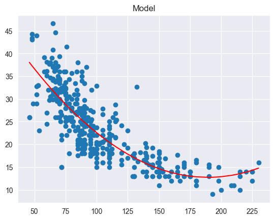
Key Points:
Used when relationship between and is non-linear
Still a linear model (linear in parameters !)
Can fit using standard least squares
Degree determined by:
Residual plots (check if pattern remains)
Cross-validation
Hypothesis tests (is significant?)
Example: captures non-linear relationship
Warning: High-degree polynomials can overfit!
Model Selection
Variable Selection Methods
Best Subset Selection:
Fit all possible models (with predictors)
For each size , choose best model (lowest RSS or highest )
Select single best model using criterion (AIC, BIC, adj-, )
Problem: Computationally infeasible for
BIC and AIC Scorers for Linear Regression Model Selection
from statsmodels.tools.eval_measures import aic as sm_aic, bic as sm_bic

def aic_scorer(estimator, X, y):
    """
    Compute AIC for linear regression model.
    Returns negative AIC.
    """
    y_pred = estimator.predict(X)
    n = len(y) # number of observations
    k = X.shape[1] + 1  # number of parameters (features + intercept)

    res = y - y_pred
    rss = np.sum(res ** 2)

    # Log-likelihood for !!linear regression!!
    llf = -0.5 * n * (np.log(rss / n) + np.log(2 * np.pi))

    return sm_aic(llf, n, k) * -1 # because we want to maximize

def bic_scorer(estimator, X, y):
    """
    Compute BIC for linear regression model.
    Returns negative BIC (loss function).
    """
    y_pred = estimator.predict(X)
    n = len(y)  # number of observations
    k = X.shape[1] + 1  # number of parameters (features + intercept)

    res = y - y_pred
    rss = np.sum(res ** 2)

    # Log-likelihood for linear regression
    llf = -0.5 * n * (np.log(rss / n) + np.log(2 * np.pi))

    return sm_bic(llf, n, k) * -1  # because we want to maximize
Forward Stepwise Selection:
import pandas as pd
from sklearn.feature_selection import SequentialFeatureSelector
from sklearn.linear_model import LinearRegression

df = pd.read_csv('predictive-modeling/Credit.csv')
df = pd.get_dummies(data=df, drop_first=True, dtype=float)

X = df.drop(columns='Balance')
y = df['Balance']

model = LinearRegression()
sfs = SequentialFeatureSelector(
    model,
    direction="forward",   # or "backward"
    n_features_to_select="auto",  # or a number
    # Estimators have a score method providing a default evaluation criterion
    # for the problem they are designed to solve. Most commonly this is
    # accuracy for classifiers and R^2 for regressors.
    # https://scikit-learn.org/stable/modules/model_evaluation.html#scoring-api-overview
    #
    # You can use default (=None), create your own (see aic_scorer or bic_scorer), or builtin:
    # https://scikit-learn.org/stable/modules/model_evaluation.html#string-name-scorers
    scoring=aic_scorer,
)
sfs.fit(X, y)

mask = sfs.get_support()
features = X.columns[mask]
features
Index(['Income', 'Limit', 'Rating', 'Cards', 'Age', 'Student_Yes'], dtype='object')Start with (null model: only intercept)
For :
Add one predictor that most improves fit (lowest RSS)
Result:
Select single best model from using criterion
Advantage: Only models (computationally efficient)
Greedy algorithm (may miss best overall model)
Backward Stepwise Selection:
import pandas as pd
from sklearn.feature_selection import SequentialFeatureSelector
from sklearn.linear_model import LinearRegression

df = pd.read_csv('predictive-modeling/Credit.csv')
df = pd.get_dummies(data=df, drop_first=True, dtype=float)

X = df.drop(columns='Balance')
y = df['Balance']

model = LinearRegression()
sfs = SequentialFeatureSelector(
    model,
    direction="backward",   # or "forward"
    n_features_to_select="auto",  # or a number
    # Estimators have a score method providing a default evaluation criterion
    # for the problem they are designed to solve. Most commonly this is
    # accuracy for classifiers and R^2 for regressors.
    # https://scikit-learn.org/stable/modules/model_evaluation.html#scoring-api-overview
    #
    # You can use default (=None), create your own (see aic_scorer or bic_scorer), or builtin:
    # https://scikit-learn.org/stable/modules/model_evaluation.html#string-name-scorers
    scoring=aic_scorer,
)
sfs.fit(X, y)

mask = sfs.get_support()
features = X.columns[mask]
features
Index(['Income', 'Limit', 'Rating', 'Cards', 'Age', 'Student_Yes'], dtype='object')Start with (full model: all predictors)
For :
Remove predictor whose removal least hurts fit
Result:
Select single best model using criterion
Advantage: Only models
Limitation: Requires
Hybrid Stepwise Selection:
Alternates between adding and removing variables
Can correct for earlier mistakes
Similar computational efficiency to forward/backward
Model Selection Criteria
Goal: Balance fit vs. complexity (avoid overfitting)
import statsmodels.api as sm
import pandas as pd

df = pd.read_csv('predictive-modeling/Credit.csv')

def fit_model(predictors):
    X = sm.add_constant(df[predictors])
    y = df["Balance"]
    model = sm.OLS(y, X).fit()
    return model

M1 = fit_model(["Income"])
M2 = fit_model(["Income", "Limit"])
M3 = fit_model(["Income", "Limit", "Rating"])
M4 = fit_model(["Income", "Limit", "Rating", "Cards"])

models = {"M1": M1, "M2": M2, "M3": M3, "M4": M4}
Adjusted → Select model that maximizes adj-:
for name, model in models.items():
    print(name, "adj_R2 =", model.rsquared_adj)
M1 adj_R2 = 0.21300489131364186
M2 adj_R2 = 0.8704575713334397
M3 adj_R2 = 0.8753013618810308
M4 adj_R2 = 0.8757468863485864
Formula:
Regular always increases with more predictors
Adjusted penalizes adding predictors
AIC (Akaike Information Criterion) → Select model that minimizes AIC:
for name, model in models.items():
    print(name, "AIC =", model.aic)
M1 AIC = 5945.89424951724
M2 AIC = 5225.202531162302
M3 AIC = 5210.950291148072
M4 AIC = 5210.507229752486
For least squares:
General form:
: likelihood, : number of parameters
Penalty term: increases with more predictors
BIC (Bayesian Information Criterion) → Select model that minimizes BIC:
for name, model in models.items():
    print(name, "BIC =", model.bic)
M1 BIC = 5953.877178611456
M2 BIC = 5237.176924803626
M3 BIC = 5226.9161493365045
M4 BIC = 5230.464552488025
Tends to select smaller models than AIC
For least squares:
General form:
Penalty term: stronger than AIC for
Mallows’ → Select model that minimizes :
import numpy as np

def mallows_cp(model_candidate, model_full):
    """
    Mallows Cp using slide formula:
        Cp = (1/n) * (RSS_m + 2 * p * sigma_hat^2_full)
    model_candidate: statsmodels OLSResults for the subset model
    model_full:      statsmodels OLSResults for the largest model
    """
    n = model_candidate.nobs # number of observations
    RSS_m = np.sum(model_candidate.resid**2) # residual sum of squares of the candidate model

    # p = number of parameters in candidate model (including intercept)
    p = int(model_candidate.df_model) + 1

    sigma2_full = model_full.mse_resid  # estimate of the error variance σ̂² from full model

    Cp = (RSS_m + 2 * p * sigma2_full) / n
    return Cp

print(f"M1 Cp = {mallows_cp(M1, M4)}")
print(f"M2 Cp = {mallows_cp(M2, M4)}")
print(f"M3 Cp = {mallows_cp(M3, M4)}")
print(f"M4 Cp = {mallows_cp(M4, M4)}")
M1 Cp = 165784.50530352452
M2 Cp = 27571.04635232112
M3 Cp = 26620.27911254733
M4 Cp = 26592.707689604606
Formula:
Proportional to AIC for least squares
Key Insight:
All criteria balance fit (RSS) vs. complexity ()
AIC: prediction-focused
BIC: explanation-focused, stronger penalty → simpler models
For large , BIC ≈ AIC with stronger penalty
Regularization Methods
Ridge Regression
Objective Function: Minimize
###################
# Ridge Regression
###################

import pandas as pd
import numpy as np

from sklearn.preprocessing import StandardScaler
from sklearn.linear_model import Ridge

df = pd.read_csv('predictive-modeling/Credit.csv', index_col="Unnamed: 0")
df = pd.get_dummies(data=df, drop_first=True, dtype=float)

X = df.drop(columns='Balance')
# Standardize predictors (Ridge is scale-sensitive)
X = pd.DataFrame(StandardScaler().fit_transform(X), columns=X.columns, index=X.index)
y = df['Balance']

# Fit model:
lambda_ridge = 100
ridge = Ridge(alpha=lambda_ridge) # alpha = lambda
ridge.fit(X, y)

print(
    f"Ridge coefficients (λ = {lambda_ridge}):\n",
    pd.DataFrame({ "Predictor": ["**Intercept**"] + list(X.columns), "Ridge Coefficient": [ridge.intercept_] + list(ridge.coef_)})
)

#########################################
# Ridge with Cross-Validation to choose λ
#########################################

import pandas as pd
import numpy as np

from sklearn.preprocessing import StandardScaler
from sklearn.linear_model import RidgeCV

df = pd.read_csv('predictive-modeling/Credit.csv', index_col="Unnamed: 0")
df = pd.get_dummies(data=df, drop_first=True, dtype=float)

X = df.drop(columns='Balance')
# Standardize predictors (Ridge is scale-sensitive)
X = pd.DataFrame(StandardScaler().fit_transform(X), columns=X.columns, index=X.index)
y = df['Balance']

# Grid of λ values to try
alphas = np.logspace(-2, 4, 50)  # 10^-2 to 10^4
ridge_cv = RidgeCV(alphas=alphas, cv=10)
ridge_cv.fit(X, y)

print(
    f"Ridge coefficients (Cross Validation selected λ = {ridge_cv.alpha_}):\n",
    pd.DataFrame({ "Predictor": ["**Intercept**"] + list(X.columns), "Ridge Coefficient": [ridge.intercept_] + list(ridge.coef_)})
)
Ridge coefficients (λ = 100):
Predictor Ridge Coefficient
0 **Intercept** 520.015000
1 Income -94.597784
2 Limit 211.391442
3 Rating 209.601376
4 Cards 22.356504
5 Age -19.035029
6 Education -0.423652
7 Gender_Female 0.179193
8 Student_Yes 97.638749
9 Married_Yes -6.011495
10 Ethnicity_Asian 3.512579
11 Ethnicity_Caucasian 3.544476
Ridge coefficients (Cross Validation selected λ = 0.517947467923121):
Predictor Ridge Coefficient
0 **Intercept** 520.015000
1 Income -94.597784
2 Limit 211.391442
3 Rating 209.601376
4 Cards 22.356504
5 Age -19.035029
6 Education -0.423652
7 Gender_Female 0.179193
8 Student_Yes 97.638749
9 Married_Yes -6.011495
10 Ethnicity_Asian 3.512579
11 Ethnicity_Caucasian 3.544476
Components:
RSS: want good fit
: penalty (shrinkage penalty)
: tuning parameter
Behavior:
→ ordinary least squares (no penalty)
→ all (maximum shrinkage)
Intermediate : balance fit and shrinkage
Properties:
Shrinks coefficients toward zero
Does NOT set coefficients exactly to zero
All predictors remain in final model
Reduces variance at cost of increased bias
Helps with collinearity (stabilizes coefficients)
Equivalent Constrained Form: Minimize RSS subject to
Larger (or smaller ) → less shrinkage
Why standardize?
Ridge penalty depends on scale of predictors
Always standardize predictors before applying ridge
Lasso Regression
Objective Function: Minimize
##################
# Lasso Regression
##################

import pandas as pd
import numpy as np

from sklearn.preprocessing import StandardScaler
from sklearn.linear_model import Lasso

df = pd.read_csv('predictive-modeling/Credit.csv', index_col="Unnamed: 0")
df = pd.get_dummies(data=df, drop_first=True, dtype=float)

X = df.drop(columns='Balance')
# Standardize predictors (Lasso is scale-sensitive)
X = pd.DataFrame(StandardScaler().fit_transform(X), columns=X.columns, index=X.index)
y = df['Balance']

# Fit model:
lambda_lasso = 0.5
lasso = Lasso(alpha=lambda_lasso, max_iter=10000) # alpha = lambda
lasso.fit(X, y)

print(
    f"Lasso coefficients (λ = {lambda_lasso}):\n",
    pd.DataFrame({ "Predictor": ["**Intercept**"] + list(X.columns), "Lasso Coefficient": [lasso.intercept_] + list(lasso.coef_)})
)

#########################################
# Lasso with Cross-Validation to choose λ
#########################################

import pandas as pd
import numpy as np

from sklearn.preprocessing import StandardScaler
from sklearn.linear_model import LassoCV

df = pd.read_csv('predictive-modeling/Credit.csv', index_col="Unnamed: 0")
df = pd.get_dummies(data=df, drop_first=True, dtype=float)

X = df.drop(columns='Balance')
# Standardize predictors (Lasso is scale-sensitive)
X = pd.DataFrame(StandardScaler().fit_transform(X), columns=X.columns, index=X.index)
y = df['Balance']

alphas_lasso = np.logspace(-3, 1, 50)

lasso_cv = LassoCV(alphas=alphas_lasso, cv=10, max_iter=10000, random_state=0)
lasso_cv.fit(X, y)

print(
    f"Lasso coefficients (Cross Validation selected λ = {lasso_cv.alpha_}):\n",
    pd.DataFrame({ "Predictor": ["**Intercept**"] + list(X.columns), "Lasso Coefficient": [lasso_cv.intercept_] + list(lasso_cv.coef_)})
)
Lasso coefficients (λ = 0.5):
Predictor Lasso Coefficient
0 **Intercept** 520.015000
1 Income -272.379767
2 Limit 445.239368
3 Rating 168.100954
4 Cards 24.180697
5 Age -10.270095
6 Education -2.974457
7 Gender_Female -4.738478
8 Student_Yes 127.195235
9 Married_Yes -3.541359
10 Ethnicity_Asian 6.012987
11 Ethnicity_Caucasian 3.833064
Lasso coefficients (Cross Validation selected λ = 0.2329951810515372):
Predictor Lasso Coefficient
0 **Intercept** 520.015000
1 Income -273.615943
2 Limit 448.113594
3 Rating 166.512475
4 Cards 24.471506
5 Age -10.427643
6 Education -3.246318
7 Gender_Female -5.050454
8 Student_Yes 127.513394
9 Married_Yes -3.829485
10 Ethnicity_Asian 6.685630
11 Ethnicity_Caucasian 4.481290
Components:
RSS: want good fit
: penalty
: tuning parameter
Properties:
Shrinks coefficients toward zero
Sets some coefficients exactly to zero (automatic variable selection!)
Produces sparse models (only subset of predictors)
More interpretable than ridge
Also helps with collinearity
Equivalent Constrained Form: Minimize RSS subject to
Why Lasso Produces Sparse Solutions:
constraint region has corners (diamond shape in 2D)
RSS contours (ellipses) often intersect constraint at corners
At corners, some coefficients are exactly zero
Ridge has circular constraint (no corners) → no exact zeros
Comparing Ridge and Lasso
| Ridge | Lasso | |
|---|---|---|
| Penalty | : | : |
| Exact zeros? | No | Yes |
| Variable selection? | No | Yes |
| All predictors included? | Yes | No (sparse) |
| Interpretability | Lower | Higher |
| When to use | Many predictors, all relevant | Many predictors, few relevant |
Bias-Variance Trade-Off:
Both reduce variance by introducing bias
As increases: variance ↓, bias ↑
Optimal minimizes test MSE
Selecting Tuning Parameter 
Method: Cross-Validation
Choose grid of values (e.g., 10-2 to 106)
For each :
Perform -fold CV
Compute CV error (MSE for regression)
Select that minimizes CV error
Refit model on full training data with chosen
Typical Result:
too small → overfitting (high variance, acts like OLS)
too large → underfitting (high bias, coefficients too small)
Optimal in middle
Logistic Regression
import pandas as pd
import statsmodels.api as sm

df = pd.read_csv('predictive-modeling/Default.csv', sep=';')
df = df.join(pd.get_dummies(df['default'], prefix='default', drop_first=True, dtype=float))

x = df['balance']
y = df['default_Yes']

x_sm = sm.add_constant(x)

model = sm.GLM(y, x_sm, family=sm.families.Binomial()).fit()
# or: model = sm.Logit(y, x_sm).fit()

print(model.summary())
Generalized Linear Model Regression Results
==============================================================================
Dep. Variable: default_Yes No. Observations: 10000
Model: GLM Df Residuals: 9998
Model Family: Binomial Df Model: 1
Link Function: Logit Scale: 1.0000
Method: IRLS Log-Likelihood: -798.23
Date: Wed, 28 Jan 2026 Deviance: 1596.5
Time: 19:11:44 Pearson chi2: 7.15e+03
No. Iterations: 9 Pseudo R-squ. (CS): 0.1240
Covariance Type: nonrobust
==============================================================================
coef std err z P>|z| [0.025 0.975]
------------------------------------------------------------------------------
const -10.6513 0.361 -29.491 0.000 -11.359 -9.943
balance 0.0055 0.000 24.952 0.000 0.005 0.006
==============================================================================
Properties:
Output always between 0 and 1 (valid probability)
S-shaped curve
Linear relationship in log-odds scale
Odds:
Odds = 1: equal probability (50-50)
Odds : more likely is
Odds : more likely is
Log-Odds (Logit):
Linear in !
This is why it’s called “logistic regression”
Interpretation of Coefficients:
: change in log-odds for 1-unit increase in
Unit increase in → odds multiply by
: positive association ()
: negative association ()
Estimation:
Use Maximum Likelihood (not least squares!)
No closed-form solution, requires numerical optimization
Example Calculation: If , , :
log-odds
odds
import pandas as pd
import statsmodels.api as sm

df = pd.read_csv('predictive-modeling/Default.csv', sep=';')
df = pd.get_dummies(data=df, drop_first=True, dtype=float)

X = df[['balance', 'income']]
y = df['default_Yes']

X_sm = sm.add_constant(X)
model = sm.GLM(y, X_sm, family=sm.families.Binomial()).fit()
# or: model = sm.Logit(y, X_sm).fit()

print(model.summary())
Generalized Linear Model Regression Results
==============================================================================
Dep. Variable: default_Yes No. Observations: 10000
Model: GLM Df Residuals: 9997
Model Family: Binomial Df Model: 2
Link Function: Logit Scale: 1.0000
Method: IRLS Log-Likelihood: -789.48
Date: Wed, 28 Jan 2026 Deviance: 1579.0
Time: 19:11:44 Pearson chi2: 6.95e+03
No. Iterations: 9 Pseudo R-squ. (CS): 0.1256
Covariance Type: nonrobust
==============================================================================
coef std err z P>|z| [0.025 0.975]
------------------------------------------------------------------------------
const -11.5405 0.435 -26.544 0.000 -12.393 -10.688
balance 0.0056 0.000 24.835 0.000 0.005 0.006
income 2.081e-05 4.99e-06 4.174 0.000 1.1e-05 3.06e-05
==============================================================================
Interpretation:
: change in log-odds when increases by 1, holding other constant
Holding others constant, odds multiply by
Classification & Model Evaluation
Classification Rule:
If threshold (typically 0.5) → predict
If threshold → predict
Confusion Matrix:
from sklearn.metrics import confusion_matrix

threshold = 0.5
y_pred = model.predict(X_sm)
y_pred = (y_pred >= threshold).astype(int)

print(confusion_matrix(y, y_pred))

tn, fp, fn, tp = confusion_matrix(y, y_pred).ravel()
total = tn + fp + fn + tp
print(f"TN = {tn}, FP = {fp}, FN = {fn}, TP = {tp}, Total = {total}")
[[9629 38]
[ 225 108]]
TN = 9629, FP = 38, FN = 225, TP = 108, Total = 10000
                Predicted Class
              0           1
Actual  0    TN          FP    (Total N)
        1    FN          TP    (Total P)
TP (True Positive): correctly predicted 1
TN (True Negative): correctly predicted 0
FP (False Positive): predicted 1, actually 0 (Type I error)
FN (False Negative): predicted 0, actually 1 (Type II error)
Performance Metrics:
from sklearn.metrics import classification_report
from sklearn.metrics import accuracy_score, precision_score, recall_score, f1_score

threshold = 0.5
y_pred = model.predict(X_sm)
y_pred = (y_pred >= threshold).astype(int)

print(classification_report(y, y_pred))
# macro average: Simple average of precision, recall and f1-score across all classes (treats each class equally).
# weighted average: Average weighted by the number of samples in each class (accounts for class imbalance).

print(f"Accuracy Score:\t\t{accuracy_score(y, y_pred):.3f}")
print(f"Precision Score:\t{precision_score(y, y_pred):.3f}")
print(f"Recall Score:\t\t{recall_score(y, y_pred):.3f}")
# Specificity is just recall of the negative class (pos_label=0)
print(f"Specificity Score:\t{recall_score(y, y_pred, pos_label=0):.3f}")
print(f"F1-Score:\t\t\t{f1_score(y, y_pred):.3f}")
precision recall f1-score support
0.0 0.98 1.00 0.99 9667
1.0 0.74 0.32 0.45 333
accuracy 0.97 10000
macro avg 0.86 0.66 0.72 10000
weighted avg 0.97 0.97 0.97 10000
Accuracy Score: 0.974
Precision Score: 0.740
Recall Score: 0.324
Specificity Score: 0.996
F1-Score: 0.451
Accuracy
Proportion of correct predictions
Problem: Misleading with class imbalance!
Precision
Among predicted positives, what fraction are correct?
High precision: few false alarms
Recall (Sensitivity, True Positive Rate)
Among actual positives, what fraction did we detect?
High recall: catch most positives
Specificity (True Negative Rate)
Among actual negatives, what fraction did we correctly identify?
F1 Score
Harmonic mean of precision and recall
Balances both metrics
Good for imbalanced classes
False Positive Rate
Classification Error
Receiver Operating Characteristic (ROC) Curve
from sklearn.metrics import roc_curve, roc_auc_score
import matplotlib.pyplot as plt

y_pred = model.predict(X_sm)

fpr, tpr, thresholds = roc_curve(y, y_pred)
auc = roc_auc_score(y, y_pred)

# Plot
plt.figure(figsize=(6, 5))
plt.plot(fpr, tpr, label=f"AUC = {auc:.4f}")
plt.plot([0, 1], [0, 1], "k--", label="Random classifier")
for i in range(len(thresholds)): # Annotate some thresholds on the curve
    if i % 100 == 0:
        plt.annotate(
            text=f"{thresholds[i]:.2f}",
            xy=(fpr[i], tpr[i]),
            xytext=(-30, 15),
            textcoords='offset points',
            arrowprops=dict(arrowstyle='->', lw=0.5),
            bbox=dict(boxstyle='round,pad=0.3', facecolor='yellow', alpha=0.5)
        )
plt.xlabel("False Positive Rate")
plt.ylabel("True Positive Rate (Recall)")
plt.title("ROC Curve")
plt.legend()
plt.grid(alpha=0.3)
plt.tight_layout()
plt.show()

fpr_threshold = 0.05 # lte
tpr_threshold = 0.7 # gte
for i in range(len(thresholds)):
    if fpr[i] <= fpr_threshold and tpr[i] >= tpr_threshold:
        print(f"i = {i}:\tThreshold = {thresholds[i]:.4f}, True Positive Rate = {tpr[i]:.4f}, False Positive Rate: {fpr[i]:.2f}")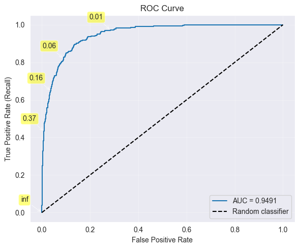
i = 228:	Threshold = 0.1299, True Positive Rate = 0.7027, False Positive Rate: 0.05
i = 229:	Threshold = 0.1268, True Positive Rate = 0.7027, False Positive Rate: 0.05
i = 230:	Threshold = 0.1266, True Positive Rate = 0.7057, False Positive Rate: 0.05
i = 231:	Threshold = 0.1237, True Positive Rate = 0.7057, False Positive Rate: 0.05
i = 232:	Threshold = 0.1225, True Positive Rate = 0.7087, False Positive Rate: 0.05
i = 233:	Threshold = 0.1218, True Positive Rate = 0.7087, False Positive Rate: 0.05
i = 234:	Threshold = 0.1217, True Positive Rate = 0.7117, False Positive Rate: 0.05
i = 235:	Threshold = 0.1213, True Positive Rate = 0.7117, False Positive Rate: 0.05
i = 236:	Threshold = 0.1211, True Positive Rate = 0.7147, False Positive Rate: 0.05
i = 237:	Threshold = 0.1182, True Positive Rate = 0.7147, False Positive Rate: 0.05
i = 238:	Threshold = 0.1181, True Positive Rate = 0.7177, False Positive Rate: 0.05
Receiver Operating Characteristic (ROC) Curve:
Plot True Positive Rate (Recall) vs False Positive Rate
Each point corresponds to different threshold
Ideal: Curve hugs top-left corner (high TPR, low FPR)
Baseline: Diagonal line (random classifier)
Area Under Curve (AUC):
AUC = 1: perfect classifier
AUC = 0.5: random classifier
AUC : good classifier
Using ROC to Choose Threshold:
High threshold → low FPR, low TPR (conservative)
Low threshold → high FPR, high TPR (liberal)
Choose threshold based on cost of FP vs FN
Class Imbalance Problem
###############
# Down-sampling
###############

import numpy as np
import pandas as pd
import statsmodels.api as sm

np.random.seed(0)

df = pd.read_csv('predictive-modeling/Default.csv', sep=';')
df = pd.get_dummies(data=df, drop_first=True, dtype=float)

i_yes = df.loc[df['default_Yes'] == 1, :].index
i_no = df.loc[df['default_Yes'] == 0, :].index

if len(i_yes) < len(i_no):
    i_no = np.random.choice(i_no, replace=False, size=len(i_yes))
else:
    i_yes = np.random.choice(i_yes, replace=False, size=len(i_no))

i_all = np.concatenate((i_no, i_yes))

x = df.iloc[i_all]['balance']
y = df.iloc[i_all]['default_Yes']

x_sm = sm.add_constant(x)
model = sm.GLM(y, x_sm, family=sm.families.Binomial()).fit()
# or: model = sm.Logit(y, x_sm).fit()

print("Down-sampling:")
print(f"len(Yes) = {len(i_yes)}, len(No) = {len(i_no)}, len(Total) = {len(i_all)}")
print(model.summary())

###############
# Up-sampling
###############
import numpy as np
import pandas as pd
import statsmodels.api as sm
from sklearn.utils import resample

np.random.seed(0)

df = pd.read_csv('predictive-modeling/Default.csv', sep=';')
df = pd.get_dummies(data=df, drop_first=True, dtype=float)

i_yes = df.loc[df['default_Yes'] == 1, :].index
i_no = df.loc[df['default_Yes'] == 0, :].index

if len(i_yes) > len(i_no):
    i_no = resample(
        i_no,
        replace=True,
        n_samples=len(i_yes),
        random_state=42
    )
else:
    i_yes = resample(
        i_yes,
        replace=True,
        n_samples=len(i_no),
        random_state=42
    )

i_all = np.concatenate((i_no, i_yes))

x = df.iloc[i_all]['balance']
y = df.iloc[i_all]['default_Yes']

x_sm = sm.add_constant(x)
model = sm.GLM(y, x_sm, family=sm.families.Binomial()).fit()
# or: model = sm.Logit(y, x_sm).fit()

print("\n\n\nUp-sampling:")
print(f"len(Yes) = {len(i_yes)}, len(No) = {len(i_no)}, len(Total) = {len(i_all)}")
print(model.summary())
Down-sampling:
len(Yes) = 333, len(No) = 333, len(Total) = 666
Generalized Linear Model Regression Results
==============================================================================
Dep. Variable: default_Yes No. Observations: 666
Model: GLM Df Residuals: 664
Model Family: Binomial Df Model: 1
Link Function: Logit Scale: 1.0000
Method: IRLS Log-Likelihood: -199.05
Date: Wed, 28 Jan 2026 Deviance: 398.10
Time: 19:11:45 Pearson chi2: 491.
No. Iterations: 6 Pseudo R-squ. (CS): 0.5455
Covariance Type: nonrobust
==============================================================================
coef std err z P>|z| [0.025 0.975]
------------------------------------------------------------------------------
const -7.1129 0.569 -12.495 0.000 -8.229 -5.997
balance 0.0053 0.000 13.216 0.000 0.005 0.006
==============================================================================
Up-sampling:
len(Yes) = 9667, len(No) = 9667, len(Total) = 19334
Generalized Linear Model Regression Results
==============================================================================
Dep. Variable: default_Yes No. Observations: 19334
Model: GLM Df Residuals: 19332
Model Family: Binomial Df Model: 1
Link Function: Logit Scale: 1.0000
Method: IRLS Log-Likelihood: -5672.1
Date: Wed, 28 Jan 2026 Deviance: 11344.
Time: 19:11:45 Pearson chi2: 1.75e+04
No. Iterations: 7 Pseudo R-squ. (CS): 0.5505
Covariance Type: nonrobust
==============================================================================
coef std err z P>|z| [0.025 0.975]
------------------------------------------------------------------------------
const -7.3292 0.109 -67.047 0.000 -7.544 -7.115
balance 0.0055 7.9e-05 70.269 0.000 0.005 0.006
==============================================================================
Problem Example:
Dataset: 97% class 0, 3% class 1
Trivial classifier: always predict 0
Accuracy = 97% (looks great!)
But useless: never detects class 1
Why Imbalance is Bad:
Likelihood function dominated by majority class
Model learns to predict majority class
Minority class ignored
Solutions:
Down-sampling: Randomly remove observations from majority class
Balanced classes
Loses data
Up-sampling: Replicate observations from minority class
Balanced classes
Can overfit
Adjust Threshold: Lower threshold to catch more positives
Simple
Trade-off: more false positives
Use Appropriate Metrics: Focus on F1, precision, recall (not accuracy)
Cost-Sensitive Learning: Weight observations by class
Cross-Validation for Classification
-Fold Cross-Validation / -Fold CV:
Split data into test data and training data, then split training data into k folds. Estimate the classification score by averaging across folds.
import pandas as pd
from sklearn.linear_model import LogisticRegression
from sklearn.model_selection import cross_val_score

df = pd.read_csv('predictive-modeling/Default.csv', sep=';')
df = pd.get_dummies(data=df, drop_first=True, dtype=float)

x = df[['balance']]
y = df['default_Yes']

model = LogisticRegression()

k = 5

# Default (None): Usually Accuracy (for classifiers) or $R^2$ (for regressors).
# Result: A number between 0 and 1 (e.g., 0.85 means 85% accuracy or $R^2=0.85$).
# Higher is better.
scores = cross_val_score(model, x, y, cv=k)
print(f"Estimated Classification Score: {scores.mean():.4f} (Scores = {scores})")

# Explicit "Error" Metric: If you use a scoring string starting with neg_
# (e.g., 'neg_mean_squared_error', 'neg_log_loss'), it returns negative error.
# Result: A negative number (e.g., -12.5). The closer to 0 (less negative), the better.
# Why? Sklearn always maximizes scores, so it flips errors to be negative
# (maximizing -10 is better than maximizing -20).
scores = cross_val_score(model, x, y, cv=k, scoring='neg_mean_squared_error')
print(f"Estimated Classification Error: {-scores.mean():.4f} (Errors = {-scores})")
Estimated Classification Score: 0.9725 (Scores = [0.972 0.972 0.9715 0.9735 0.9735])
Estimated Classification Error: 0.0275 (Errors = [0.028 0.028 0.0285 0.0265 0.0265])
Split data into folds (typically or 10)
For to :
Train on folds
Test on fold
Compute classification error on fold :
CV error
Leave-One-Out Cross-Validation (LOOCV):
import pandas as pd
from sklearn.linear_model import LogisticRegression
from sklearn.model_selection import LeaveOneOut, cross_val_score

df = pd.read_csv('predictive-modeling/Default.csv', sep=';')
df = pd.get_dummies(data=df, drop_first=True, dtype=float)

x = df[['balance']]
y = df['default_Yes']

model = LogisticRegression(max_iter=1000)

loo = LeaveOneOut()
scores = cross_val_score(model, x, y, cv=loo, scoring='neg_mean_squared_error')

print(f"LOOCV: {loo.get_n_splits(x)} folds (n = {len(x)})")
print(f"MSE per fold (first 10): {-scores[:10]}")
print(f"Mean MSE: {-scores.mean():.4f}")
print(f"Std MSE: {scores.std():.4f}")
LOOCV: 10000 folds (n = 10000)
MSE per fold (first 10): [0. 0. 0. 0. 0. 0. 0. 0. 0. 0.]
Mean MSE: 0.0275
Std MSE: 0.1635
Less bias, more variance
Computationally expensive for large datasets (trains models)
Purpose:
Estimate test error
Choose between models
Tune hyperparameters (e.g., threshold)
Important: Stratify folds to preserve class proportions!
Time Series: Introduction & Decomposition
Fundamental Concepts
Time Series: Observations ordered in time
Stochastic Process: Sequence of random variables
Time series is one realization (sample path) of process
Like drawing one sample from a distribution
Serial Correlation: Observations are dependent over time
Violates independence assumption of standard regression
Requires special methods
Goals:
Describe and visualize data
Model underlying process
Decompose into components (trend, seasonality, noise)
Forecast future values
Regression with time series predictors
Basic Stochastic Processes
White Noise:
import matplotlib.pyplot as plt
import numpy as np

# White noise signal
w = np.random.normal(size=1000)

# plot
fig = plt.figure(figsize=(10, 5))
ax = fig.add_subplot(1, 1, 1)
ax.plot(w)
ax.grid()
plt.xlabel("Time")
plt.ylabel("Value")

plt.show()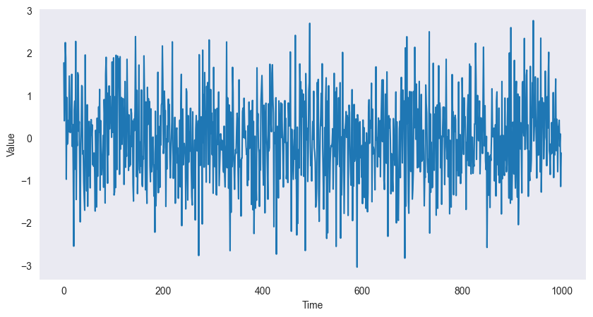
are i.i.d. with ,
No correlation: for
Completely unpredictable
ACF: for
Random Walk:
import matplotlib.pyplot as plt
import numpy as np

n_samp = 10000

# Random samples d and cumulative sum x
d = np.random.choice(a=[-1,1], size=n_samp, replace=True)
x = np.cumsum(d)

# Add drift delta
delta = 5e-2
y = np.linspace(0, n_samp * delta, n_samp)
y += x

# Plot
fig = plt.figure(figsize=(10, 5))
ax = fig.add_subplot(1, 1, 1)
ax.plot(x, label="random walk")
ax.plot(y, label="random walk with drift")
ax.grid()
plt.xlabel("Time")
plt.ylabel("y-deviation in [m]")
plt.legend()
plt.show()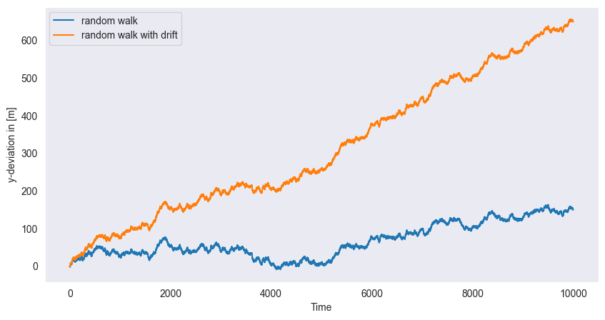
, starting
Cumulative sum:
With drift: (adds trend )
Non-stationary (variance grows with time)
(if drift),
Moving Average (MA):
import numpy as np
import pandas as pd

w = np.random.normal(size=1000)
w = pd.DataFrame(w)

# Filter with window = 3
v = w.rolling(window=3).mean()

# plot
fig = plt.figure(figsize=(10, 5))
ax = fig.add_subplot(1, 1, 1)
ax.plot(v)
ax.grid()
plt.xlabel("Time")
plt.show()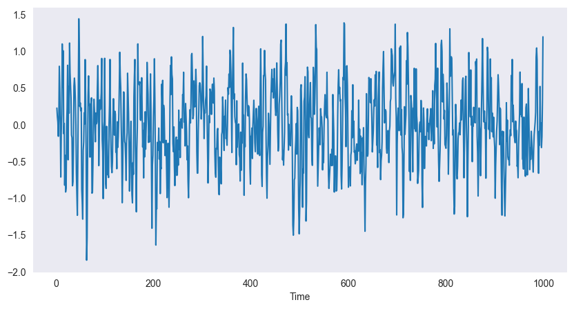
Example (3-point):
Smooths white noise
Reduces high-frequency fluctuations
Stationary
Autoregressive (AR):
import numpy as np
import pandas as pd

w = np.random.normal(size=1000)
w = pd.DataFrame(w)

# Autoregressive filter:
ar = np.zeros(1000)
for i in range(2,1000):
    ar[i] = 1.5 * ar[i-1] - 0.9 * ar[i-2] + w.iloc[i]

# plot
fig = plt.figure(figsize=(10, 5))
ax = fig.add_subplot(1, 1, 1)
ax.plot(ar)
ax.grid()
plt.xlabel("Autoregressive Process")

plt.show()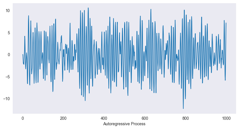
Example (AR(2)):
Current value depends on past values
Can exhibit oscillations, trends (if non-stationary)
Captures dependence structure
Stationarity
import matplotlib.pyplot as plt
import pandas as pd
from statsmodels.graphics.tsaplots import plot_acf # autocorrelation function
from statsmodels.tsa.stattools import adfuller

df = pd.read_csv('predictive-modeling/AustralianElectricity.csv', sep =";")
index = pd.DatetimeIndex(data=pd.to_datetime(df["Quarter"]), freq='infer')
df.set_index(index, inplace=True)
df.drop("Quarter", axis=1, inplace=True)

# If ACF decays very slowly, the series is likely non-stationary (has trend or seasonality).
# Else-If ACF drops quickly to within confidence bands, the series is closer to stationary.

fig, axes = plt.subplots(1, 2, figsize=(12, 4))
axes[0].plot(df.index, df["kilowatt"])
axes[0].set_title("Time Series")
axes[0].set_xlabel("Date")
axes[0].set_ylabel("Kilowatt")

plot_acf(df["kilowatt"], lags=40, ax=axes[1])
axes[1].set_title("ACF (Autocorrelation Function)")

plt.tight_layout()
plt.show()

##########################################################
# Augmented Dickey-Fuller test (formal stationarity test)
##########################################################

adfuller_results = adfuller(df["kilowatt"])
adf = adfuller_results[0]
pvalue = adfuller_results[1]
critical_values = adfuller_results[4]

print("ADF Statistic:", adf, "\np-value:", pvalue, "\nCritical Values:")
for key, value in critical_values.items():
    print(f"  {key}: {value}")

if pvalue < 0.05:
    print("Reject H₀: Series is stationary")
else:
    print("Fail to reject H₀: Series is non-stationary")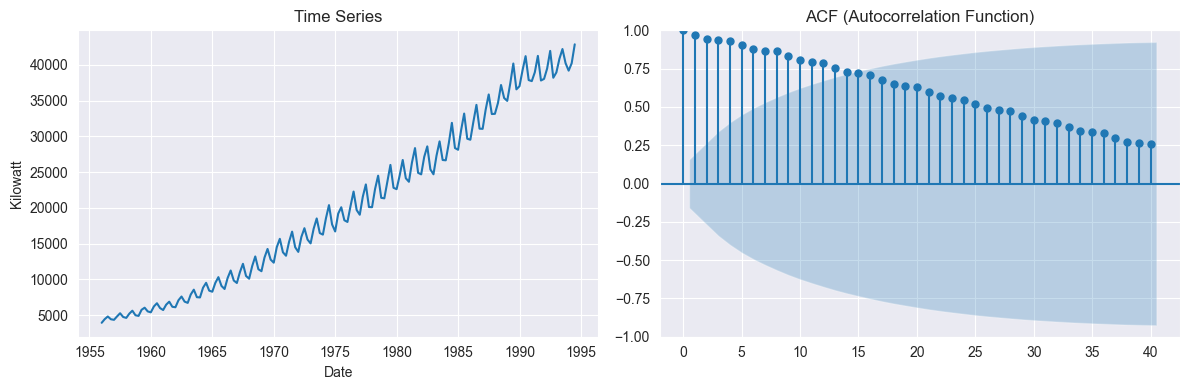
ADF Statistic: -0.27312130644566773
p-value: 0.9292258325376282
Critical Values:
  1%: -3.4776006742422374
  5%: -2.882265832283648
  10%: -2.5778219289774156
Fail to reject H₀: Series is non-stationary
Strict Stationarity:
Joint distribution unchanged by time shifts
For any , and have same distribution
Too strong for practice
Weak Stationarity (Second-Order Stationarity): Two conditions:
Constant mean: for all
Autocovariance depends only on lag:
for all
Doesn’t depend on absolute time , only lag
Why Weak Stationarity Matters:
Allows statistical inference from single time series
Can estimate autocovariance from one realization
Most models assume weak stationarity
Non-Stationary Indicators:
Trend (increasing/decreasing mean)
Changing variance over time
Seasonality (periodic pattern)
ACF decays very slowly
Stationarity for a Time Series requires three conditions:
Constant mean: (independent of )
Constant variance: (independent of )
Autocovariance depends only on lag: (independent of )
For ARMA processes, a simpler criterion exists: the characteristic equation (or equivalently, checking the roots of the characteristic polynomial).
Proof Method 1: Characteristic Equation (Most Direct)
Convention 1: Rewrite the AR(2) process in lag operator notation:
Rearrange to Standard Form (move all terms to the left side):
The characteristic equation is obtained by replacing with :
Multiply by :
This is the standard form for the quadratic formula: ,
for which: , , .
# Coefficients in descending order of power:
np.abs(np.roots([1, -1/2, -1/3]))
array([0.87915287, 0.37915287])Both roots satisfy (they lie inside the unit circle). Since both roots of the characteristic polynomial lie strictly inside the unit circle, the AR(2) process is stationary.
Convention 2: Rewrite the AR(2) process into its Characteristic Polynomial:
Rearrange to Standard Form (move all terms to the left side):
Introduce the Lag Operator (Backshift Operator):
Define the lag operator such that: , , and rewrite the equation using :
Factor out on the left:
This is the lag polynomial form:
where
Direct Polynomial Substitution: Replace with , set equal to zero and rearrange to standard form (coefficients in descending order of power):
Stationarity condition: All roots satisfy
# Coefficients in descending order of power:
np.abs(np.roots([0.1, 1/2, -1/2, 1]))
array([6.09052833, 1.28136399, 1.28136399])Solve Manually for roots using the quadratic formula:
Numerically: , so
Proof Method 2: Verification via Mean (Supporting Proof)
Assuming stationarity, let . Taking expectations of both sides:
The mean is well-defined and constant at , consistent with stationarity.
Autocovariance & Autocorrelation Functions
Theoretical Autocovariance Function (ACOVF):
import numpy as np
import pandas as pd
from statsmodels.tsa.stattools import acovf # autocovariance function

np.random.seed(0)

w = np.random.normal(size=1000, loc=2, scale=0.1)
w = pd.DataFrame(w)
w = w.rolling(window=3).mean()

gamma = acovf(w, adjusted=False, missing='drop', fft=False)
n_lags = 50  # Plot first n lags, use len(gamma) - 1 for all lags

plt.figure(figsize=(10, 4))
plt.stem(range(n_lags+1), gamma[:n_lags+1], basefmt=" ")
plt.axhline(0, color='black', linewidth=0.8)
plt.xlabel("Lag h")
plt.ylabel("Autocovariance γ(h)")
plt.title(f"Autocovariance Function (ACVF) - First {n_lags} lags")
plt.grid(alpha=0.3)
plt.tight_layout()
plt.show()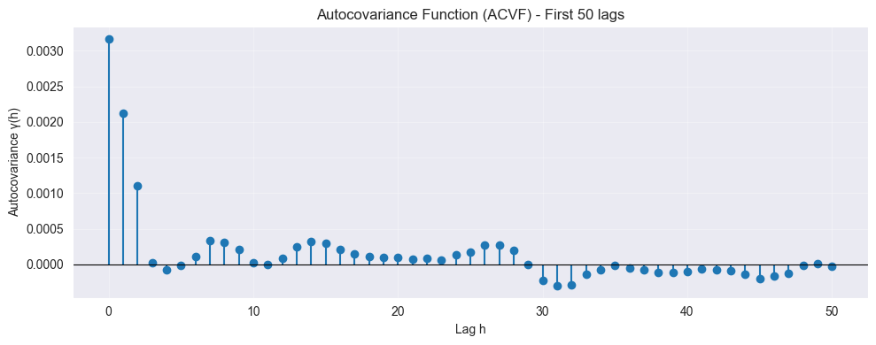
(symmetric)
Sample Autocovariance:
Theoretical Autocorrelation Function (ACF):
import numpy as np
import pandas as pd

from statsmodels.tsa.stattools import acf # autocorrelation function
from statsmodels.graphics.tsaplots import plot_acf # plot autocorrelation function

np.random.seed(0)

w = np.random.normal(size=1000, loc=2, scale=0.1)
w = pd.DataFrame(w)
w = w.rolling(window=3).mean()

fig = plt.figure(figsize=(10, 5))
ax = fig.add_subplot(1, 1, 1)
plot_acf(w, missing='drop', lags=50, ax=ax, c='C1')
plt.xlabel("Lag")
plt.ylabel("Autocorrelation")
plt.show()

print(f"Autocorrelation = {acf(w, missing='drop', nlags=3 - 1, fft=True)}")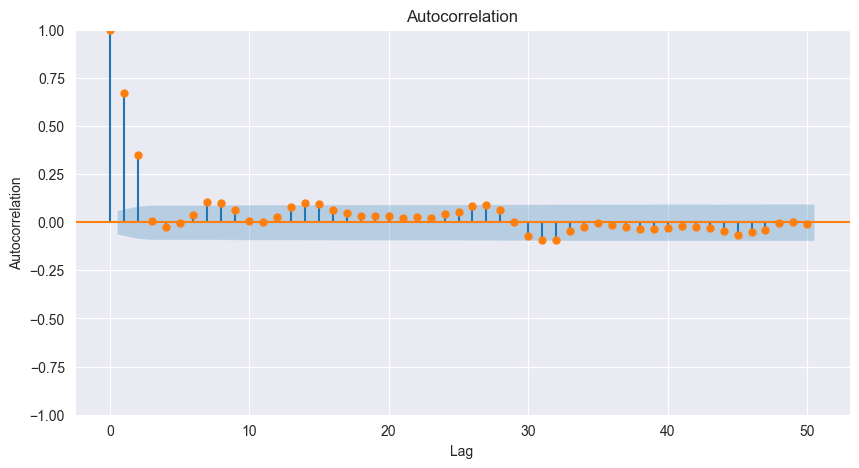
Autocorrelation = [1. 0.67030704 0.34969521]
Measures linear dependence at lag
Sample Autocorrelation:
White Noise ACF:
For white noise with large : for
95% confidence bands:
If for all → consistent with white noise
Interpretation:
: no linear relationship at lag
: positive correlation (peaks followed by peaks)
: negative correlation (peaks followed by troughs)
Transformations
Purpose: Achieve stationarity, stabilize variance, reduce skewness
Box-Cox Transformation:
import pandas as pd
import matplotlib.pyplot as plt
from scipy.stats import boxcox

df = pd.read_csv('predictive-modeling/AirPassengers.csv', parse_dates=True)
index = pd.DatetimeIndex(data=pd.to_datetime(df["TravelDate"]), freq='infer')
df.set_index(index, inplace=True)
df.drop("TravelDate", axis=1, inplace=True)

# Apply Box-Cox transformation (requires positive data)
y_positive = df["Passengers"] - df["Passengers"].min() + 1  # Shift to make positive
y_boxcox, lambda_opt = boxcox(y_positive)

print(f"Optimal λ: {lambda_opt:.4f}")

fig, axes = plt.subplots(1, 2, figsize=(12, 4))
axes[0].plot(df.index, y_positive, label="Original")
axes[0].set_title("Original Series")
axes[0].set_ylabel("Value")

axes[1].plot(df.index, y_boxcox, label="Box-Cox Transformed", color="orange")
axes[1].set_title(f"Box-Cox Transformed (λ={lambda_opt:.2f})")
axes[1].set_ylabel("Transformed Value")

plt.tight_layout()
plt.show()
Optimal λ: 0.4818
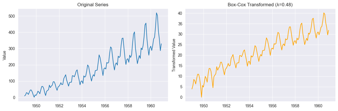
g(x) = (x^λ - 1)/λ   if λ ≠ 0
g(x) = log(x) if λ = 0: no transformation
: square root
: logarithm
: reciprocal
Choose to stabilize variance and reduce skewness
Differencing:
import numpy as np
import pandas as pd
import matplotlib.pyplot as plt

# Generate synthetic monthly time series with trend and seasonality
np.random.seed(42)

n = 120  # 10 years of monthly data
time = pd.date_range(start='2014-01', periods=n, freq='MS')

# Trend + Seasonality + Noise
trend = np.linspace(10, 30, n)
seasonal = 5 * np.sin(2 * np.pi * np.arange(n) / 12)  # 12-month cycle
noise = np.random.normal(scale=1.5, size=n)
y = trend + seasonal + noise

df = pd.DataFrame({"date": time, "value": y})
df.set_index("date", inplace=True)

df["diff1"] = df["value"].diff()

fig, axes = plt.subplots(2, 1, figsize=(10, 6))

axes[0].plot(df.index, df["value"])
axes[0].set_title("Original Series")
axes[0].set_ylabel("Value")

axes[1].plot(df.index, df["diff1"])
axes[1].set_title("First Difference (removes trend)")
axes[1].set_ylabel("Δ Value")
axes[1].axhline(0, color='red', linestyle='--', linewidth=0.8)

plt.tight_layout()
plt.show()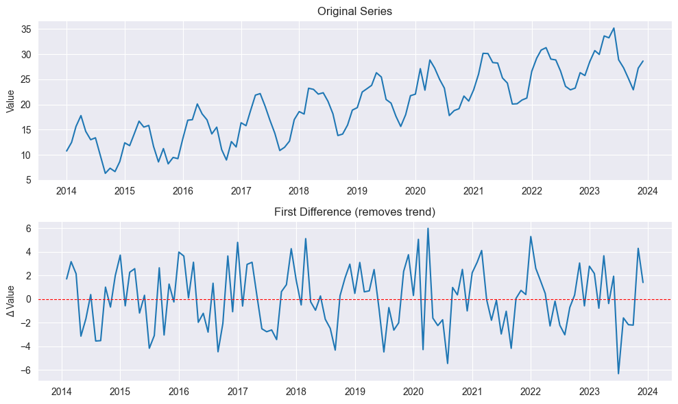
First difference:
Removes linear trend
Backshift operator:
Differencing operator:
Second difference:
Seasonal Differencing:
import numpy as np
import pandas as pd
import matplotlib.pyplot as plt

# Generate synthetic monthly time series with trend and seasonality
np.random.seed(42)

n = 120  # 10 years of monthly data
time = pd.date_range(start='2014-01', periods=n, freq='MS')

# Trend + Seasonality + Noise
trend = np.linspace(10, 30, n)
seasonal = 5 * np.sin(2 * np.pi * np.arange(n) / 12)  # 12-month cycle
noise = np.random.normal(scale=1.5, size=n)
y = trend + seasonal + noise

df = pd.DataFrame({"date": time, "value": y})
df.set_index("date", inplace=True)

# Seasonal difference (12-month period)
df["seasonal_diff"] = df["value"].diff(12)

fig, axes = plt.subplots(2, 1, figsize=(10, 6))

axes[0].plot(df.index, df["value"])
axes[0].set_title("Original Series")
axes[0].set_ylabel("Value")

axes[1].plot(df.index, df["seasonal_diff"], label="Seasonal Difference (lag=12)")
axes[1].set_title("Seasonal Differencing")
axes[1].set_ylabel("Δ Value")
axes[1].axhline(0, color='red', linestyle='--', linewidth=0.8)

plt.show()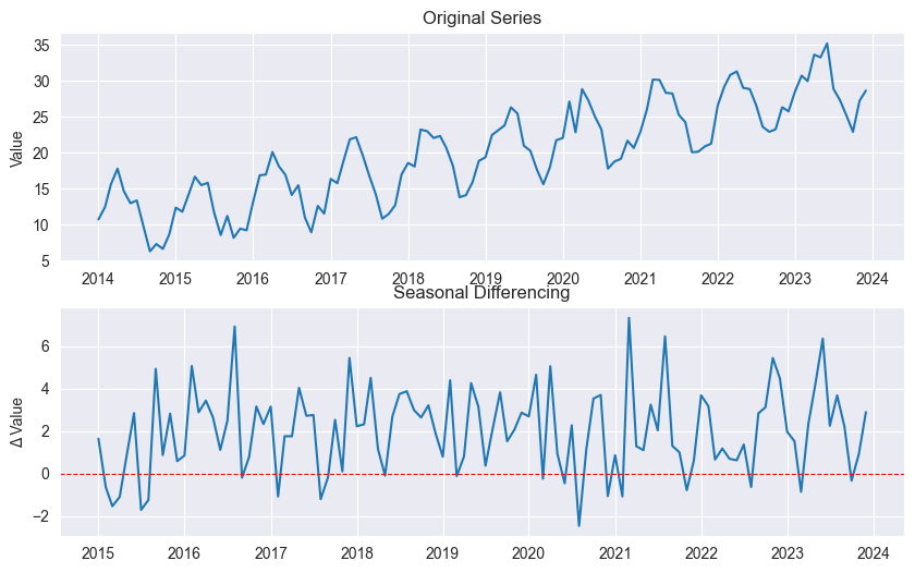
( = seasonal period, e.g., for monthly)
Removes seasonal pattern
Log-Returns (Finance):
Approximates relative change:
Often stationary even when prices non-stationary
Time Series Decomposition
Additive Model:
import numpy as np
import pandas as pd
from statsmodels.tsa.seasonal import seasonal_decompose
import matplotlib.pyplot as plt

# Generate synthetic monthly time series with trend and seasonality
np.random.seed(42)

n = 120  # 10 years of monthly data
time = pd.date_range(start='2014-01', periods=n, freq='MS')

# Trend + Seasonality + Noise
trend = np.linspace(10, 30, n)
seasonal = 5 * np.sin(2 * np.pi * np.arange(n) / 12)  # 12-month cycle
noise = np.random.normal(scale=1.5, size=n)
y = trend + seasonal + noise

df = pd.DataFrame({"date": time, "value": y})
df.set_index("date", inplace=True)

# Additive decomposition
decomposition = seasonal_decompose(df["value"], model='additive', period=12)

fig = decomposition.plot()
fig.set_size_inches(10, 8)
plt.tight_layout()
plt.show()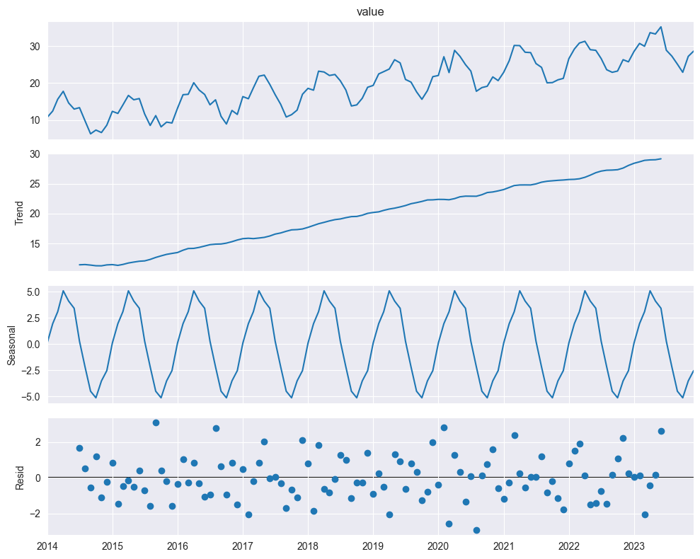
: trend component
: seasonal component
: remainder (irregular, noise)
When to use additive:
Seasonal variation roughly constant over time
Multiplicative Model:
import numpy as np
import pandas as pd
from statsmodels.tsa.seasonal import seasonal_decompose
import matplotlib.pyplot as plt

# Generate synthetic monthly time series with trend and seasonality
np.random.seed(42)

n = 120  # 10 years of monthly data
time = pd.date_range(start='2014-01', periods=n, freq='MS')

# Trend + Seasonality + Noise
trend = np.linspace(10, 30, n)
seasonal = 5 * np.sin(2 * np.pi * np.arange(n) / 12)  # 12-month cycle
noise = np.random.normal(scale=1.5, size=n)
y = trend + seasonal + noise

df = pd.DataFrame({"date": time, "value": y})
df.set_index("date", inplace=True)

# Additive decomposition
decomposition = seasonal_decompose(df["value"], model='multiplicative', period=12)

fig = decomposition.plot()
fig.set_size_inches(10, 8)
plt.tight_layout()
plt.show()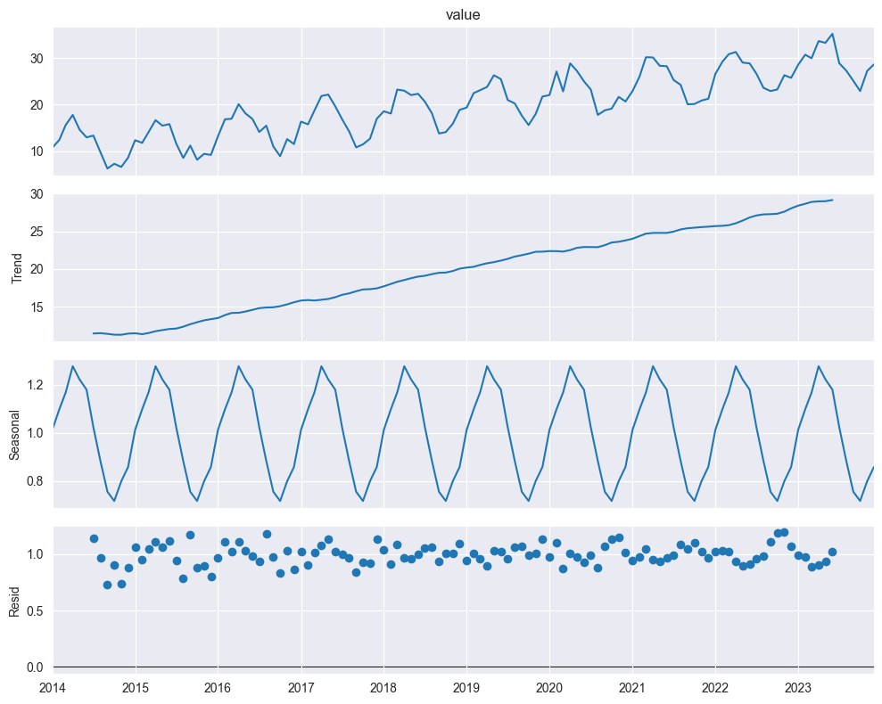
When to use multiplicative:
Seasonal variation grows/shrinks with trend
Can take logs: (additive!)
Classical Decomposition (Moving Average Method):
Estimate Trend :
Apply moving average filter of length (= seasonal period)
For monthly data (): average over 12 months
Smooths out seasonality
Estimate Seasonal Effect :
Compute detrended series:
For each position in cycle (e.g., each month):
Average all detrended values at that position
Result: seasonal pattern that repeats
Estimate Remainder :
Should be random (no structure)
Moving Average Filter:
For odd :
For even :
STL (Seasonal-Trend Decomposition using Loess):
import numpy as np
import pandas as pd
from statsmodels.tsa.seasonal import STL
import matplotlib.pyplot as plt

# Generate synthetic monthly time series with trend and seasonality
np.random.seed(42)

n = 120  # 10 years of monthly data
time = pd.date_range(start='2014-01', periods=n, freq='MS')

# Trend + Seasonality + Noise
trend = np.linspace(10, 30, n)
seasonal = 5 * np.sin(2 * np.pi * np.arange(n) / 12)  # 12-month cycle
noise = np.random.normal(scale=1.5, size=n)
y = trend + seasonal + noise

# STL decomposition
stl = STL(df["value"], period=12, seasonal=13)  # seasonal window must be odd
result = stl.fit()

fig = result.plot()
fig.set_size_inches(10, 8)
plt.tight_layout()
plt.show()

trend_stl = result.trend
seasonal_stl = result.seasonal
residual_stl = result.resid

print("Trend (first 5):", trend_stl[:5].values)
print("Seasonal (first 5):", seasonal_stl[:5].values)
print("Residual (first 5):", residual_stl[:5].values)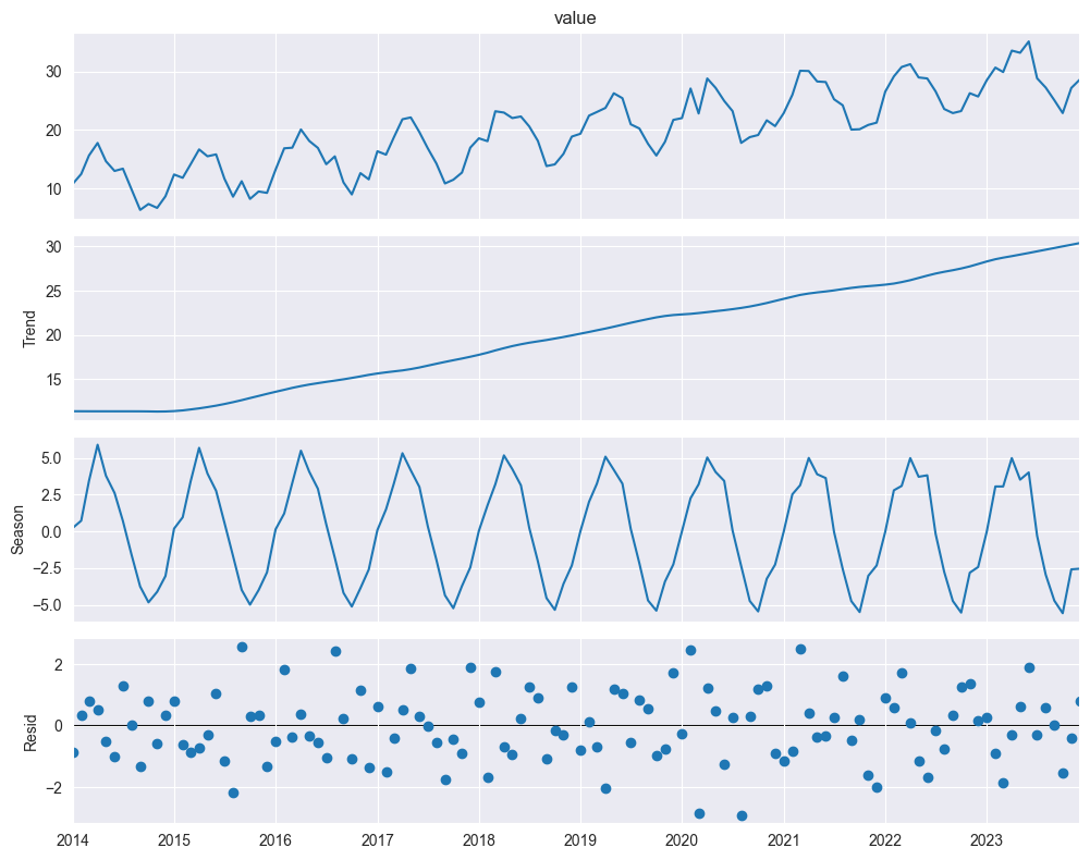
Trend (first 5): [11.3892355  11.386162   11.38341052 11.38170419 11.38106562]
Seasonal (first 5): [0.22258345 0.72413073 3.43459021 5.89856111 3.7861149 ]
Residual (first 5): [-0.86674771  0.35037805  0.81979354  0.50848116 -0.51601466]
More flexible than classical decomposition
Uses loess (local regression) instead of moving averages
Seasonal component can change over time
Robust to outliers
Iterative procedure
Advantages of STL:
Handles any type of seasonality
Seasonal component can vary slowly
Robustness to unusual observations
More accurate trend and seasonal estimates
Time Series: AR, MA, ARMA & ARIMA Models
import numpy as np
import matplotlib.pyplot as plt
from statsmodels.graphics.tsaplots import plot_acf, plot_pacf

np.random.seed(42)

# Generate white noise
n = 200
z = np.random.normal(loc=0, scale=1, size=n)

fig, axes = plt.subplots(1, 3, figsize=(15, 4))

# Time series plot
axes[0].plot(z)
axes[0].set_title("White Noise")
axes[0].set_xlabel("Time")
axes[0].set_ylabel("Value")
axes[0].axhline(0, color='red', linestyle='--', linewidth=0.8)

# Autocorrelation Function
plot_acf(z, lags=40, ax=axes[1])
axes[1].set_title("Autocorrelation Function of White Noise")

# Partial Autocorrelation Function
plot_pacf(z, lags=40, ax=axes[2])
axes[2].set_title("Partial Autocorrelation Function of White Noise")

plt.tight_layout()
plt.show()
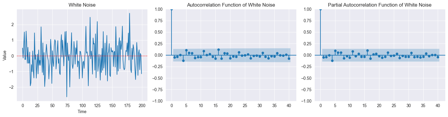
Autoregressive Model AR()
Definition:
: order (number of lagged terms)
: AR coefficients
: white noise with variance
AR Operator & Characteristic Polynomial:
Characteristic polynomial:
Stationarity Condition:
All roots of must satisfy
Equivalently: all zeros outside unit circle in complex plane
AR(1) Example:
from statsmodels.tsa.arima_process import ArmaProcess

########################
# Simulate AR(1) process
#########################
# AR(1): x_n = 0.7 * x_{n-1} + z_n
phi = [1, -0.7]  # [1, -φ₁] format; Stationarity requires |φ₁| < 1
theta = [1]      # MA coefficients (none for pure AR)

arma_process = ArmaProcess(phi, theta)

# Check stationarity
print("Is stationary?", arma_process.isstationary)
print("Is invertible?", arma_process.isinvertible)

# Simulate AR(1)
np.random.seed(42)

data = arma_process.generate_sample(nsample=200)

# Plot
fig, axes = plt.subplots(1, 3, figsize=(15, 4))

axes[0].plot(data)
axes[0].set_title("AR(1) with φ1=0.7")
axes[0].set_xlabel("Time")
axes[0].set_ylabel("Value")

plot_acf(data, lags=40, ax=axes[1])
axes[1].set_title("ACF (exponential decay)")

plot_pacf(data, lags=40, ax=axes[2])
axes[2].set_title("PACF (cuts off after lag 1)")

plt.tight_layout()
plt.show()

###################################
# Estimate AR(1) using statsmodels
###################################

from statsmodels.tsa.arima.model import ARIMA

# Fit AR(1) model: ARIMA(1,0,0)
model = ARIMA(data, order=(1, 0, 0)).fit()

print(model.summary())
Is stationary? True
Is invertible? True
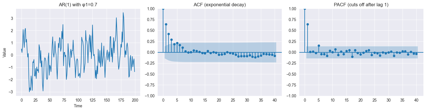
                               SARIMAX Results
==============================================================================
Dep. Variable:                      y   No. Observations:                  200
Model:                 ARIMA(1, 0, 0)   Log Likelihood                -268.801
Date:                Wed, 28 Jan 2026   AIC                            543.602
Time:                        19:12:39   BIC                            553.497
Sample:                             0   HQIC                           547.606
                                - 200
Covariance Type:                  opg
==============================================================================
                 coef    std err          z      P>|z|      [0.025      0.975]
------------------------------------------------------------------------------
const         -0.1257      0.187     -0.670      0.503      -0.493       0.242
ar.L1          0.6478      0.056     11.570      0.000       0.538       0.757
sigma2         0.8585      0.086      9.974      0.000       0.690       1.027
===================================================================================
Ljung-Box (L1) (Q):                   0.00   Jarque-Bera (JB):                 0.80
Prob(Q):                              0.97   Prob(JB):                         0.67
Heteroskedasticity (H):               0.98   Skew:                             0.15
Prob(H) (two-sided):                  0.92   Kurtosis:                         3.01
===================================================================================

Warnings:
[1] Covariance matrix calculated using the outer product of gradients (complex-step).
Stationary if
Variance:
ACF: (exponential decay)
PACF: , for
AR(2) Example:
########################
# Simulate AR(2) process
########################
phi = [1, -0.5, -0.3]  # [1, -φ₁, -φ₂]
theta = [1]

arma_process = ArmaProcess(phi, theta)
print("AR(2) is stationary?", arma_process.isstationary)

data = arma_process.generate_sample(nsample=200, scale=1.0)

fig, axes = plt.subplots(1, 3, figsize=(15, 4))

axes[0].plot(data)
axes[0].set_title("AR(2) with φ1=0.5, φ2=0.3")

plot_acf(data, lags=40, ax=axes[1])
axes[1].set_title("ACF")

plot_pacf(data, lags=40, ax=axes[2])
axes[2].set_title("PACF (cuts off after lag 2)")

plt.tight_layout()
plt.show()

###################################
# Estimate AR(1) using statsmodels
###################################

from statsmodels.tsa.arima.model import ARIMA

# Fit AR(2) model: ARIMA(2,0,0)
model = ARIMA(data, order=(2, 0, 0)).fit()

print(model.summary())
AR(2) is stationary? True
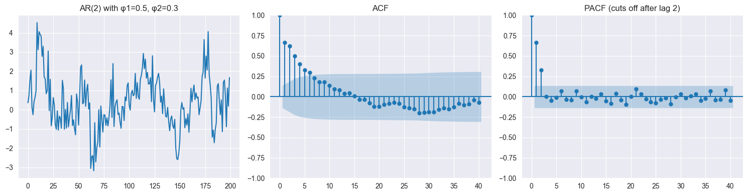
                               SARIMAX Results
==============================================================================
Dep. Variable:                      y   No. Observations:                  200
Model:                 ARIMA(2, 0, 0)   Log Likelihood                -280.673
Date:                Wed, 28 Jan 2026   AIC                            569.346
Time:                        19:12:40   BIC                            582.539
Sample:                             0   HQIC                           574.685
                                - 200
Covariance Type:                  opg
==============================================================================
                 coef    std err          z      P>|z|      [0.025      0.975]
------------------------------------------------------------------------------
const          0.4153      0.305      1.362      0.173      -0.182       1.013
ar.L1          0.4462      0.066      6.715      0.000       0.316       0.576
ar.L2          0.3237      0.067      4.799      0.000       0.192       0.456
sigma2         0.9655      0.083     11.624      0.000       0.803       1.128
===================================================================================
Ljung-Box (L1) (Q):                   0.00   Jarque-Bera (JB):                 6.20
Prob(Q):                              0.99   Prob(JB):                         0.05
Heteroskedasticity (H):               0.65   Skew:                             0.20
Prob(H) (two-sided):                  0.08   Kurtosis:                         3.77
===================================================================================

Warnings:
[1] Covariance matrix calculated using the outer product of gradients (complex-step).
Characteristic polynomial:
Find roots, check
ACF Pattern for AR():
Exponential decay (possibly with oscillations)
Tails off gradually
No clear cutoff
PACF Pattern for AR():
Cuts off after lag
, for
Use PACF to identify order !
Partial Autocorrelation:
Correlation after removing effect of intermediate lags
For AR(): equals coefficient
Moving Average Model MA()
Definition:
: order (number of lagged noise terms)
: MA coefficients
: white noise
MA Operator:
Key Property: MA processes are always stationary
Mean:
Variance:
Invertibility Condition:
All roots of must satisfy
Ensures unique MA representation
Allows writing MA as infinite AR
MA(1) Example:
########################
# Simulate MA(1) process
########################
# MA(1): x_n = z_n + 0.6*z_{n-1}
phi = [1]       # No AR part
theta = [1, 0.6]  # [1, θ₁] # Invertibility requires |θ₁| < 1

arma_process = ArmaProcess(phi, theta)
print("Is invertible?", arma_process.isinvertible)

np.random.seed(42)
data = arma_process.generate_sample(nsample=200)

fig, axes = plt.subplots(1, 3, figsize=(15, 4))

axes[0].plot(data)
axes[0].set_title("MA(1) with θ1=0.6")

plot_acf(data, lags=40, ax=axes[1])
axes[1].set_title("ACF (cuts off after lag 1)")

plot_pacf(data, lags=40, ax=axes[2])
axes[2].set_title("PACF (exponential decay)")

plt.tight_layout()
plt.show()

################
# Estimate MA(1)
################

model = ARIMA(data, order=(0, 0, 1)).fit()
print(model.summary())
Is invertible? True
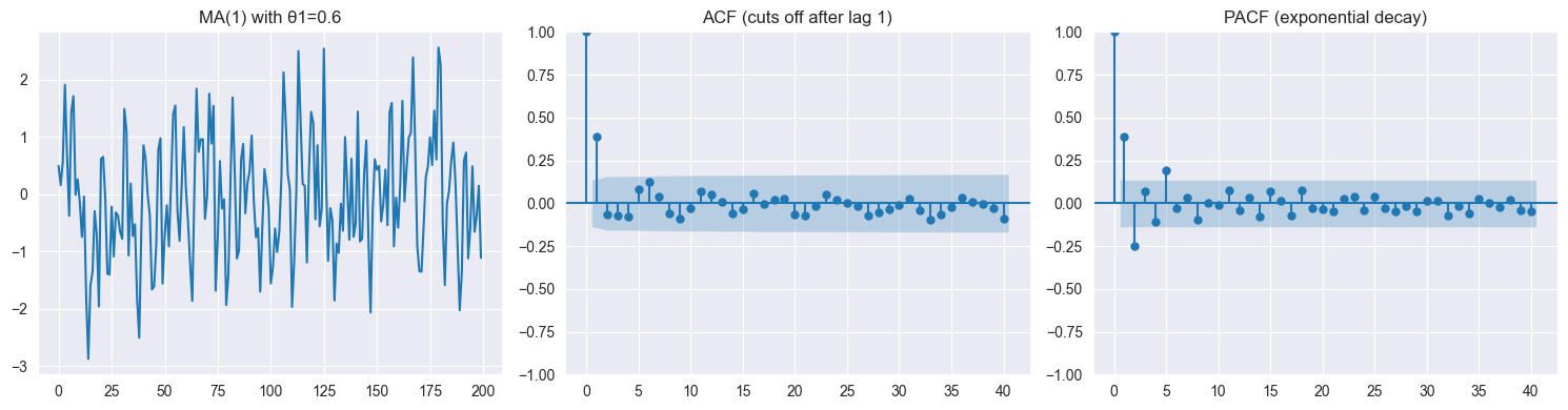
                               SARIMAX Results
==============================================================================
Dep. Variable:                      y   No. Observations:                  200
Model:                 ARIMA(0, 0, 1)   Log Likelihood                -269.176
Date:                Wed, 28 Jan 2026   AIC                            544.352
Time:                        19:12:40   BIC                            554.247
Sample:                             0   HQIC                           548.357
                                - 200
Covariance Type:                  opg
==============================================================================
                 coef    std err          z      P>|z|      [0.025      0.975]
------------------------------------------------------------------------------
const         -0.0641      0.106     -0.604      0.546      -0.272       0.144
ma.L1          0.6081      0.057     10.647      0.000       0.496       0.720
sigma2         0.8621      0.087      9.884      0.000       0.691       1.033
===================================================================================
Ljung-Box (L1) (Q):                   0.70   Jarque-Bera (JB):                 0.60
Prob(Q):                              0.40   Prob(JB):                         0.74
Heteroskedasticity (H):               1.00   Skew:                             0.13
Prob(H) (two-sided):                  0.98   Kurtosis:                         3.01
===================================================================================

Warnings:
[1] Covariance matrix calculated using the outer product of gradients (complex-step).
Variance:
ACF: , for
Invertible if
ACF Pattern for MA():
Cuts off after lag
for
for
Use ACF to identify order !
PACF Pattern for MA():
Exponential decay (possibly with oscillations)
Tails off gradually
No clear cutoff
ARMA() Model
Definition:
Or:
Expanded:
Properties:
Combines AR and MA components
More flexible than pure AR or MA
Fewer parameters than pure AR or MA
Stationarity: All roots of satisfy Invertibility: All roots of satisfy
ACF & PACF Patterns:
Both tail off (no clear cutoff in either)
Hard to identify orders and from ACF/PACF alone
Use information criteria (AIC, BIC)
Model Selection Strategy:
Plot ACF and PACF
If ACF cuts off → MA()
If PACF cuts off → AR()
If both tail off → ARMA()
For ARMA, try grid of values
Choose model with lowest AIC or BIC
Estimation:
Maximum likelihood method
Iterative numerical optimization
Software:
statsmodels(Python),forecast(R)
#####################
# Simulate ARMA(1,1)
#####################

# ARMA(1,1): x_n = 0.6*x_{n-1} + z_n + 0.4*z_{n-1}
phi = [1, -0.6]  # AR part
theta = [1, 0.4]  # MA part

arma_process = ArmaProcess(phi, theta)
print("Stationary?", arma_process.isstationary)
print("Invertible?", arma_process.isinvertible)

np.random.seed(42)
data = arma_process.generate_sample(nsample=200)

fig, axes = plt.subplots(1, 3, figsize=(15, 4))

axes[0].plot(data)
axes[0].set_title("ARMA(1,1)")

plot_acf(data, lags=40, ax=axes[1])
axes[1].set_title("ACF (exponential decay)")

plot_pacf(data, lags=40, ax=axes[2])
axes[2].set_title("PACF (exponential decay)")

plt.tight_layout()
plt.show()


#####################
# Estimate ARMA(1,1)
#####################
model = ARIMA(data, order=(1, 0, 1)).fit()
print(model.summary())
Stationary? True
Invertible? True
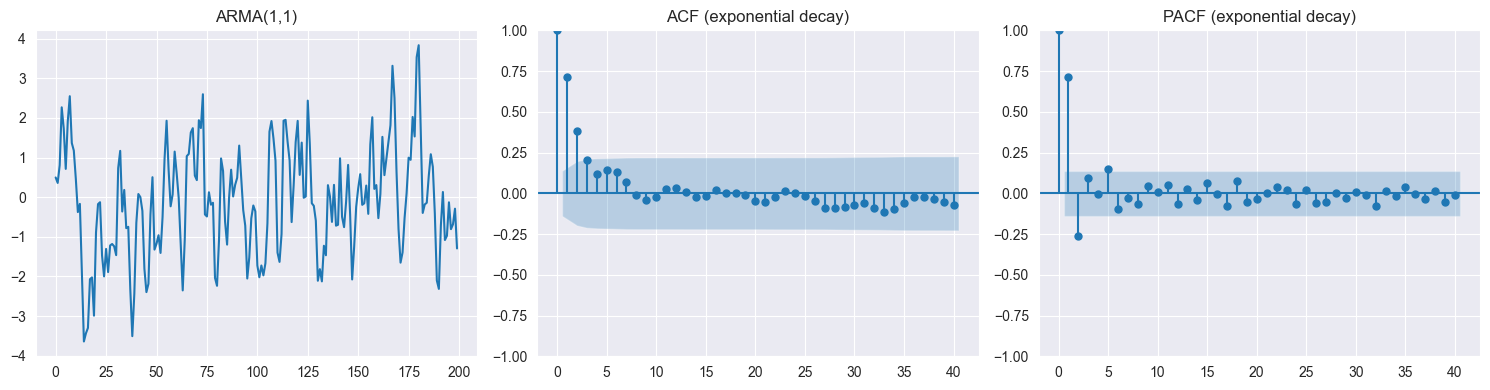
                               SARIMAX Results
==============================================================================
Dep. Variable:                      y   No. Observations:                  200
Model:                 ARIMA(1, 0, 1)   Log Likelihood                -268.841
Date:                Wed, 28 Jan 2026   AIC                            545.682
Time:                        19:12:41   BIC                            558.875
Sample:                             0   HQIC                           551.021
                                - 200
Covariance Type:                  opg
==============================================================================
                 coef    std err          z      P>|z|      [0.025      0.975]
------------------------------------------------------------------------------
const         -0.1340      0.197     -0.679      0.497      -0.521       0.253
ar.L1          0.5204      0.086      6.074      0.000       0.352       0.688
ma.L1          0.4313      0.088      4.885      0.000       0.258       0.604
sigma2         0.8572      0.086      9.915      0.000       0.688       1.027
===================================================================================
Ljung-Box (L1) (Q):                   0.01   Jarque-Bera (JB):                 0.84
Prob(Q):                              0.94   Prob(JB):                         0.66
Heteroskedasticity (H):               0.98   Skew:                             0.16
Prob(H) (two-sided):                  0.93   Kurtosis:                         3.04
===================================================================================

Warnings:
[1] Covariance matrix calculated using the outer product of gradients (complex-step).
ARIMA() Model
Purpose: Model non-stationary series
Definition:
: degree of differencing
: differencing operator
: difference times
Idea:
Original series non-stationary
Difference times to get stationary series
Fit ARMA() to
Result: ARIMA() for
Common Cases:
ARIMA() = ARMA() (already stationary)
ARIMA(): First-difference, then ARMA
ARIMA(): Random walk ()
ARIMA() with drift: Random walk with drift
ARIMA(): Local linear trend model
Model Building Process (Box-Jenkins):
###########################################
# Generate non-stationary data with trend
###########################################
import pandas as pd

# Create series with trend
np.random.seed(42)
n = 150
time = np.arange(n)
trend = 0.5 * time  # Linear trend
seasonal = 3 * np.sin(2 * np.pi * time / 12)
noise = np.random.normal(scale=2, size=n)
ts_nonstationary = trend + seasonal + noise

plt.figure(figsize=(10, 4))
plt.plot(ts_nonstationary)
plt.title("Non-stationary Time Series (trend + seasonality)")
plt.xlabel("Time")
plt.ylabel("Value")
plt.grid(alpha=0.3)
plt.tight_layout()
plt.show()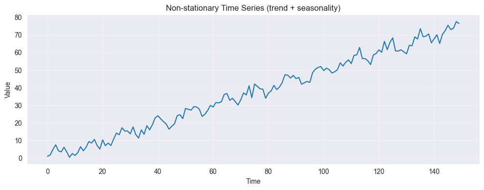
Build Automatically
#########################################
# Auto ARIMA (automated model selection)
#########################################
from pmdarima import auto_arima

# Automatically find best ARIMA model
auto_model = auto_arima(ts_nonstationary,
                        start_p=0, max_p=3,
                        start_q=0, max_q=3,
                        start_d=0, max_d=2,
                        seasonal=False,
                        stepwise=True,
                        suppress_warnings=True,
                        information_criterion='aic',
                        trace=True)

print("Best model selected by auto_arima:")
print(auto_model.summary())
Performing stepwise search to minimize aic
ARIMA(0,1,0)(0,0,0)[0] intercept : AIC=748.970, Time=0.00 sec
ARIMA(1,1,0)(0,0,0)[0] intercept : AIC=731.428, Time=0.01 sec
ARIMA(0,1,1)(0,0,0)[0] intercept : AIC=730.964, Time=0.01 sec
ARIMA(0,1,0)(0,0,0)[0] : AIC=751.321, Time=0.00 sec
ARIMA(1,1,1)(0,0,0)[0] intercept : AIC=732.799, Time=0.01 sec
ARIMA(0,1,2)(0,0,0)[0] intercept : AIC=732.950, Time=0.01 sec
ARIMA(1,1,2)(0,0,0)[0] intercept : AIC=734.778, Time=0.02 sec
ARIMA(0,1,1)(0,0,0)[0] : AIC=739.573, Time=0.00 sec
Best model: ARIMA(0,1,1)(0,0,0)[0] intercept
Total fit time: 0.063 seconds
Best model selected by auto_arima:
SARIMAX Results
==============================================================================
Dep. Variable: y No. Observations: 150
Model: SARIMAX(0, 1, 1) Log Likelihood -362.482
Date: Wed, 28 Jan 2026 AIC 730.964
Time: 19:12:41 BIC 739.976
Sample: 0 HQIC 734.626
- 150
Covariance Type: opg
==============================================================================
coef std err z P>|z| [0.025 0.975]
------------------------------------------------------------------------------
intercept 0.5050 0.141 3.573 0.000 0.228 0.782
ma.L1 -0.3771 0.082 -4.604 0.000 -0.538 -0.217
sigma2 7.5884 1.091 6.955 0.000 5.450 9.727
===================================================================================
Ljung-Box (L1) (Q): 0.00 Jarque-Bera (JB): 3.09
Prob(Q): 0.97 Prob(JB): 0.21
Heteroskedasticity (H): 1.26 Skew: -0.09
Prob(H) (two-sided): 0.42 Kurtosis: 2.32
===================================================================================
Warnings:
[1] Covariance matrix calculated using the outer product of gradients (complex-step).
Build Manually
Identify :
Plot time series
Check ACF (slow decay suggests non-stationarity)
Difference until stationary
Use Dickey-Fuller test
Typically , or 2
##################################
# Check stationarity with ADF test
##################################

from statsmodels.tsa.stattools import adfuller

def adf_test(series, name=""):
    result = adfuller(series.dropna())
    print(f"ADF Test: {name}")
    print(f"ADF Statistic: {result[0]:.4f}")
    print(f"p-value: {result[1]:.4f}")
    print(f"Critical Values:")
    for key, value in result[4].items():
        print(f"  {key}: {value:.3f}")

    if result[1] < 0.05:
        print("Reject H₀: Series is STATIONARY")
    else:
        print("Fail to reject H₀: Series is NON-STATIONARY")
    return result[1]

# Test original series
adf_test(pd.Series(ts_nonstationary), "Original Series")

################################
# Apply differencing and retest
################################

# First difference
ts_diff1 = pd.Series(ts_nonstationary).diff().dropna()

fig, axes = plt.subplots(2, 1, figsize=(10, 6))

axes[0].plot(ts_nonstationary)
axes[0].set_title("Original (Non-stationary)")
axes[0].set_ylabel("Value")

axes[1].plot(ts_diff1)
axes[1].set_title("After 1st Difference")
axes[1].set_ylabel("Δ Value")
axes[1].axhline(0, color='red', linestyle='--', linewidth=0.8)

plt.tight_layout()
plt.show()

# Test differenced series
adf_test(ts_diff1, "After 1st Difference")
ADF Test: Original Series
ADF Statistic: 0.2500
p-value: 0.9749
Critical Values:
1%: -3.479
5%: -2.883
10%: -2.578
Fail to reject H₀: Series is NON-STATIONARY

ADF Test: After 1st Difference
ADF Statistic: -8.1117
p-value: 0.0000
Critical Values:
  1%: -3.479
  5%: -2.883
  10%: -2.578
Reject H₀: Series is STATIONARY
1.2212397339380835e-12Identify and :
Plot ACF and PACF of differenced series
Determine candidate models
Try grid search
#########################################
# Plot ACF and PACF of differenced series
#########################################

fig, axes = plt.subplots(1, 3, figsize=(15, 4))

axes[0].plot(ts_diff1)
axes[0].set_title("Differenced Time Series")

plot_acf(ts_diff1, lags=40, ax=axes[1])
axes[1].set_title("ACF")

plot_pacf(ts_diff1, lags=40, ax=axes[2])
axes[2].set_title("PACF")

plt.tight_layout()
plt.show()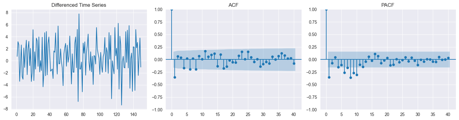
Estimate parameters:
Fit candidate models
Use maximum likelihood
from statsmodels.tsa.arima.model import ARIMA

#########################
# Fit ARIMA(1,1,1) model
#########################
# ARIMA(1,1,1): AR(1) + 1 difference + MA(1)
model = ARIMA(ts_nonstationary, order=(1, 1, 1)).fit()
print(model.summary())
SARIMAX Results
==============================================================================
Dep. Variable: y No. Observations: 150
Model: ARIMA(1, 1, 1) Log Likelihood -367.059
Date: Wed, 28 Jan 2026 AIC 740.119
Time: 19:12:42 BIC 749.130
Sample: 0 HQIC 743.780
- 150
Covariance Type: opg
==============================================================================
coef std err z P>|z| [0.025 0.975]
------------------------------------------------------------------------------
ar.L1 -0.2920 0.261 -1.117 0.264 -0.804 0.220
ma.L1 -0.0205 0.274 -0.075 0.940 -0.557 0.516
sigma2 8.0720 1.205 6.699 0.000 5.710 10.434
===================================================================================
Ljung-Box (L1) (Q): 0.58 Jarque-Bera (JB): 3.40
Prob(Q): 0.45 Prob(JB): 0.18
Heteroskedasticity (H): 1.23 Skew: -0.13
Prob(H) (two-sided): 0.46 Kurtosis: 2.31
===================================================================================
Warnings:
[1] Covariance matrix calculated using the outer product of gradients (complex-step).
Diagnose:
Check residuals (should be white noise)
ACF of residuals should be within confidence bands
Ljung-Box test
from statsmodels.tsa.arima.model import ARIMA

# Use the fitted ARIMA(1,1,1) model
model = ARIMA(ts_nonstationary, order=(1, 1, 1)).fit()
residuals = model.resid

fig, axes = plt.subplots(2, 2, figsize=(12, 8))

# Residuals plot
axes[0, 0].plot(residuals)
axes[0, 0].axhline(0, color='red', linestyle='--')
axes[0, 0].set_title("Residuals")
axes[0, 0].set_ylabel("Residual")

# Histogram
axes[0, 1].hist(residuals, bins=30, edgecolor='black', alpha=0.7)
axes[0, 1].set_title("Histogram of Residuals")
axes[0, 1].set_xlabel("Residual")

# ACF of residuals
plot_acf(residuals, lags=40, ax=axes[1, 0])
axes[1, 0].set_title("ACF of Residuals")

# Q-Q plot
from scipy import stats
stats.probplot(residuals, dist="norm", plot=axes[1, 1])
axes[1, 1].set_title("Q-Q Plot")

plt.tight_layout()
plt.show()

#############################################
# Ljung-Box test for residual autocorrelation
#############################################

from statsmodels.stats.diagnostic import acorr_ljungbox

lb_test = acorr_ljungbox(residuals, lags=20, return_df=True)
print(lb_test.head(10))
print("\nIf p-values > 0.05, residuals are white noise (good model fit)")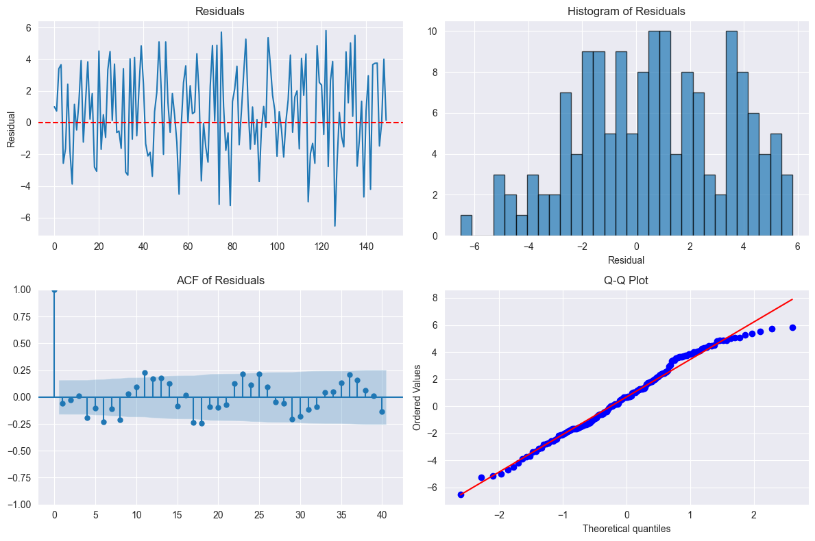
      lb_stat  lb_pvalue
1    0.577286   0.447378
2    0.676034   0.713183
3    0.689716   0.875620
4    6.361086   0.173756
5    8.017060   0.155298
6   16.240125   0.012522
7   18.111711   0.011476
8   25.348353   0.001357
9   25.472304   0.002491
10  27.015155   0.002590

If p-values > 0.05, residuals are white noise (good model fit)
Select best model:
Compare AIC or BIC
Choose simplest model with good fit
from statsmodels.tsa.arima.model import ARIMA

models = [
    (1, 1, 0),
    (1, 1, 1),
    (2, 1, 0),
    (0, 1, 1),
    (2, 1, 1),
    (1, 1, 2)
]

results = []
for order in models:
    try:
        model = ARIMA(ts_nonstationary, order=order)
        fitted = model.fit()
        results.append({
            'Order': f"ARIMA{order}",
            'AIC': fitted.aic,
            'BIC': fitted.bic,
            'Log-Likelihood': fitted.llf
        })
    except:
        pass

df_results = pd.DataFrame(results)
df_results = df_results.sort_values('AIC')
print(df_results.to_string(index=False))

print("\nBest model by AIC:", df_results.iloc[0]['Order'])
print("Best model by BIC:", df_results.sort_values('BIC').iloc[0]['Order'])
Order AIC BIC Log-Likelihood
ARIMA(1, 1, 0) 738.128061 744.135954 -367.064030
ARIMA(0, 1, 1) 739.573497 745.581390 -367.786749
ARIMA(2, 1, 0) 740.112690 749.124529 -367.056345
ARIMA(1, 1, 1) 740.118535 749.130373 -367.059267
ARIMA(1, 1, 2) 741.428986 753.444771 -366.714493
ARIMA(2, 1, 1) 742.119743 754.135528 -367.059871
Best model by AIC: ARIMA(1, 1, 0)
Best model by BIC: ARIMA(1, 1, 0)
Forecast:
Use selected model for prediction
Forecasting with AR()
-step Ahead Forecast:
Principle:
Replace future with forecasts
Replace future with their expectation (zero)
import pandas as pd
from statsmodels.tsa.arima.model import ARIMA

model = ARIMA(ts_nonstationary, order=(1, 1, 1)).fit()

# Forecast next 20 steps
forecast_steps = 20
forecast = model.get_forecast(steps=forecast_steps)
forecast_ci = pd.DataFrame(forecast.conf_int())

# Predict 50-100
prediction_start = 50
prediction_end = 100
prediction = model.get_prediction(start=prediction_start, end=prediction_end - 1)
prediction_ci = pd.DataFrame(prediction.conf_int())

######
# Plot
######
plt.figure(figsize=(12, 5))
plt.plot(ts_nonstationary, label="Observed", color='blue')

# In-sample Prediction
plt.plot(
    range(prediction_start, prediction_end),
    prediction.predicted_mean,
    label='Prediction',
    color='orange',
    linestyle='--')
plt.fill_between(
    range(prediction_start, prediction_end),
    prediction_ci.iloc[:, 0],
    prediction_ci.iloc[:, 1],
    color='yellow',
    alpha=0.3,
    label='95% CI')

# Out-of-sample Forecast
forecast_index = np.arange(len(ts_nonstationary), len(ts_nonstationary) + forecast_steps)
plt.plot(forecast_index, forecast.predicted_mean, label="Forecast", color='red', linestyle='--')
plt.fill_between(forecast_index,
                 forecast_ci.iloc[:, 0],
                 forecast_ci.iloc[:, 1],
                 color='pink', alpha=0.3, label='95% CI')
plt.legend()
plt.title("ARIMA: In-sample Prediction and Out-of-sample Forecast")
plt.xlabel("Time")
plt.ylabel("Value")
plt.grid(alpha=0.3)
plt.tight_layout()
plt.show()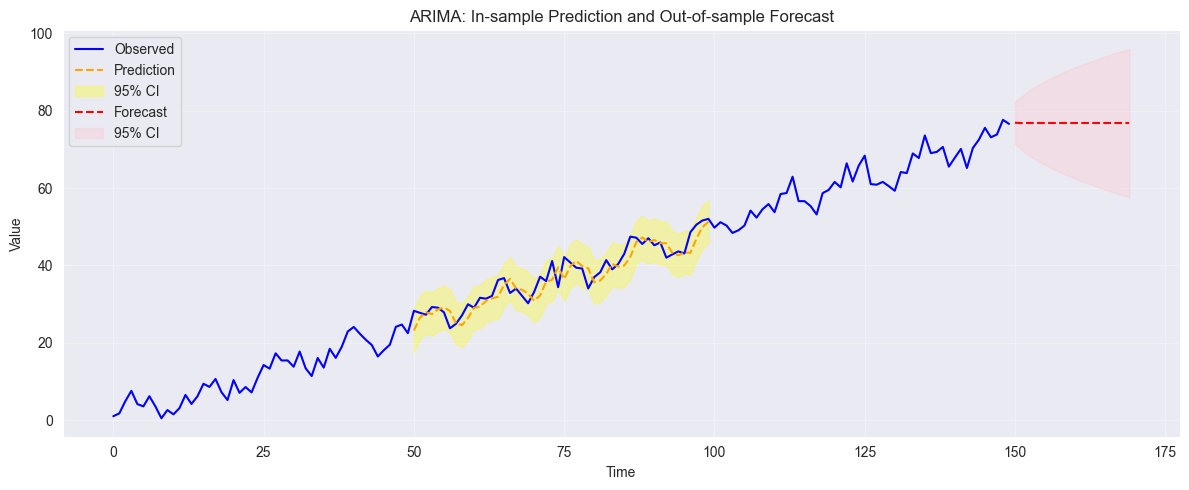
AR(1) Forecasting:
1-step:
2-step:
-step:
AR() Forecasting:
1-step:
-step: Use recursive substitution
Long-Term Behavior:
For stationary AR: (mean) as
Forecasts converge to unconditional mean
Can only predict short-term structure
Forecast Standard Error:
increases with
as
Confidence Intervals:
95% CI:
Widen as increases
Eventually cover entire range of process
SARIMA Models
import pandas as pd
from statsmodels.tsa.statespace.sarimax import SARIMAX

# Fit SARIMA
model = SARIMAX(ts_nonstationary, order=(1,1,1), seasonal_order=(1,1,1,12))
model = model.fit(disp=False)

# Forecast next 20 steps
forecast_steps = 20
forecast = model.get_forecast(steps=forecast_steps)
forecast_ci = pd.DataFrame(forecast.conf_int())

# Predict 50-100
prediction_start = 50
prediction_end = 100
prediction = model.get_prediction(start=prediction_start, end=prediction_end - 1)
prediction_ci = pd.DataFrame(prediction.conf_int())

######
# Plot
######
plt.figure(figsize=(12, 5))
plt.plot(ts_nonstationary, label="Observed", color='blue')

# In-sample Prediction
plt.plot(
    range(prediction_start, prediction_end),
    prediction.predicted_mean,
    label='Prediction',
    color='orange',
    linestyle='--')
plt.fill_between(
    range(prediction_start, prediction_end),
    prediction_ci.iloc[:, 0],
    prediction_ci.iloc[:, 1],
    color='yellow',
    alpha=0.3,
    label='95% CI')

# Out-of-sample Forecast
forecast_index = np.arange(len(ts_nonstationary), len(ts_nonstationary) + forecast_steps)
plt.plot(forecast_index, forecast.predicted_mean, label="Forecast", color='red', linestyle='--')
plt.fill_between(forecast_index,
                 forecast_ci.iloc[:, 0],
                 forecast_ci.iloc[:, 1],
                 color='pink', alpha=0.3, label='95% CI')
plt.legend()
plt.title("SARIMA: In-sample Prediction and Out-of-sample Forecast")
plt.xlabel("Time")
plt.ylabel("Value")
plt.grid(alpha=0.3)
plt.tight_layout()
plt.show()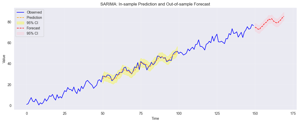
Purpose: Model series with seasonality
SARIMA(:
: non-seasonal part
: seasonal part
: seasonal period (e.g., 12 for monthly, 4 for quarterly)
Full Model:
Components:
: non-seasonal AR
: seasonal AR
: non-seasonal MA
: seasonal MA
: non-seasonal differencing
: seasonal differencing
Example: SARIMA(
Common Models:
SARIMA(: Airline model (classic for seasonal data)
SARIMA(: Pure seasonal AR
Model Selection:
Look for seasonal spikes in ACF/PACF at lags
Try grid search over
Use AIC/BIC to compare models
Performance Metrics for Time Series
import numpy as np
from statsmodels.tsa.arima.model import ARIMA

np.random.seed(42)

# Generate time series with trend and seasonality
n = 150
time = np.arange(n)
trend = 0.3 * time
seasonal = 5 * np.sin(2 * np.pi * time / 12)
noise = np.random.normal(scale=2, size=n)
y = 50 + trend + seasonal + noise

# Train-test split
train_size = 120
train = y[:train_size]
test = y[train_size:]

# Fit ARIMA model
model = ARIMA(train, order=(1, 1, 1)).fit()

# Forecast
forecast = model.forecast(steps=len(test))

print(f"Train size: {len(train)}")
print(f"Test size: {len(test)}")
print(f"Forecast shape: {forecast.shape}")
Train size: 120
Test size: 30
Forecast shape: (30,)
Mean Absolute Error (MAE):
from sklearn.metrics import mean_absolute_error
mean_absolute_error(test, forecast)6.433608462087063Average absolute forecast error
Units of original data
Robust to outliers
Minimizing MAE → forecast median
Root Mean Squared Error (RMSE):
from sklearn.metrics import mean_squared_error
np.sqrt(mean_squared_error(test, forecast))7.777461141918905Square root of average squared error
Units of original data
Penalizes large errors more than MAE
More sensitive to outliers
Minimizing RMSE → forecast mean
Mean Absolute Percentage Error (MAPE):
from sklearn.metrics import mean_absolute_percentage_error
mape = mean_absolute_percentage_error(test, forecast) * 100

if mape < 10:
    print(f"Excellent forecast; MAPE = {mape}")
elif mape < 20:
    print(f"Good forecast; MAPE = {mape}")
elif mape < 50:
    print(f"Reasonable forecast; MAPE = {mape}")
else:
    print(f"Poor forecast; MAPE = {mape}")
Excellent forecast; MAPE = 6.8575562666930905
Average absolute percentage error
Scale-independent (can compare across series)
Problem: Undefined if , extreme if
Which to Use:
MAE: Simple, interpretable, robust
RMSE: Standard in many fields, penalizes large errors
MAPE: Compare across different scales
All should be computed on test set (out-of-sample)!
from sklearn.metrics import (mean_squared_error, mean_absolute_error,
                             mean_absolute_percentage_error, r2_score)

def evaluate_forecast(y_true, y_pred, model_name="Model"):
    """Calculate all performance metrics"""
    mse = mean_squared_error(y_true, y_pred)
    rmse = np.sqrt(mse)
    mae = mean_absolute_error(y_true, y_pred)
    mape = mean_absolute_percentage_error(y_true, y_pred) * 100
    r2 = r2_score(y_true, y_pred)

    print(f"Performance Metrics: {model_name}")
    print(f"MSE:    {mse:.4f}")
    print(f"RMSE:   {rmse:.4f}")
    print(f"MAE:    {mae:.4f}")
    print(f"MAPE:   {mape:.2f}%")
    print(f"R²:     {r2:.4f}")

    return {
        'MSE': mse,
        'RMSE': rmse,
        'MAE': mae,
        'MAPE': mape,
        'R2': r2
    }

# Evaluate
metrics = evaluate_forecast(test, forecast, "ARIMA(1,1,1)")
Performance Metrics: ARIMA(1,1,1)
MSE: 60.4889
RMSE: 7.7775
MAE: 6.4336
MAPE: 6.86%
R²: -1.5123
Spectral Analysis (Brief Overview)
import numpy as np
import matplotlib.pyplot as plt

# Create signal with multiple frequencies
np.random.seed(42)
n = 500
t = np.linspace(0, 10, n)

# Signal = sum of sine waves at different frequencies
f1, f2, f3 = 2, 5, 10  # Hz
signal = (2 * np.sin(2 * np.pi * f1 * t) +
          1.5 * np.sin(2 * np.pi * f2 * t) +
          0.8 * np.sin(2 * np.pi * f3 * t) +
          np.random.normal(scale=0.5, size=n))

plt.figure(figsize=(12, 4))
plt.plot(t, signal)
plt.title('Time Series with Multiple Frequencies (2Hz, 5Hz, 10Hz)')
plt.xlabel('Time (seconds)')
plt.ylabel('Amplitude')
plt.grid(alpha=0.3)
plt.tight_layout()
plt.show()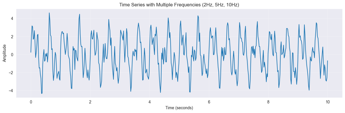
Fourier Series
Purpose: Decompose periodic function into sum of sines and cosines
import numpy as np

# Compute FFT
fft = np.fft.fft(signal) / len(signal)
fft_freq = np.fft.fftfreq(len(signal), d=(t[1]-t[0]))

# Get magnitude (power)
fft_magnitude = np.abs(fft)

# Plot only positive frequencies
positive_freq_idx = fft_freq > 0

plt.figure(figsize=(12, 5))
plt.plot(fft_freq[positive_freq_idx], fft_magnitude[positive_freq_idx])
plt.title('FFT: Frequency Spectrum')
plt.xlabel('Frequency (Hz)')
plt.ylabel('Magnitude')
plt.grid(alpha=0.3)
plt.axvline(f1, color='red', linestyle='--', alpha=0.5, label='2 Hz')
plt.axvline(f2, color='green', linestyle='--', alpha=0.5, label='5 Hz')
plt.axvline(f3, color='blue', linestyle='--', alpha=0.5, label='10 Hz')
plt.legend()
plt.tight_layout()
plt.show()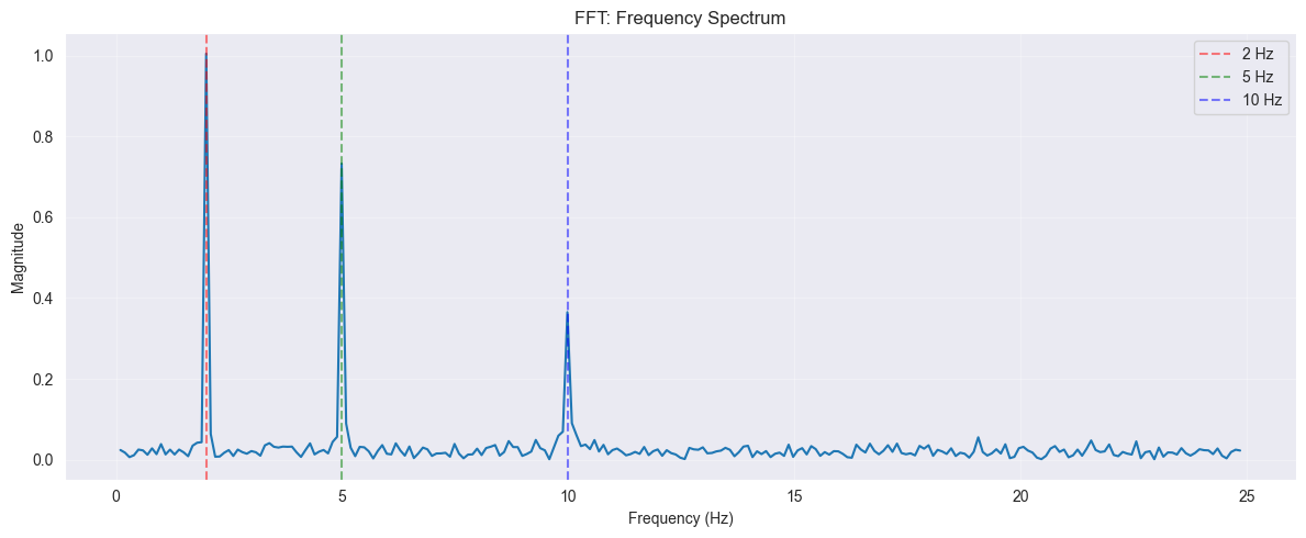
Fourier Series (period ):
Fourier Coefficients:
(average value)
Interpretation:
Each term represents harmonic at frequency
Coefficients show strength of each frequency
Discrete Fourier Transform (DFT)
For discrete series :
FFT (Fast Fourier Transform):
Efficient algorithm for computing DFT
Complexity: instead of
Standard in practice
Power Spectrum (Periodogram):
Shows strength of each frequency component
Peak at frequency → periodic component with period
Spectral Density
Continuous Spectrum:
: spectral density function
Related to autocovariance via Fourier transform
Properties:
White noise: flat spectrum (all frequencies equal)
AR/MA: smooth spectrum with peaks/troughs
Strong peak at → dominant periodic component
Use in Practice:
Identify dominant frequencies (periodicities)
Compare models (theoretical vs empirical spectrum)
Detect hidden periodic components