Advanced Statistical Data Analysis
Notebook Cell
# Install BiocManager (if not already installed)
if (!requireNamespace("BiocManager", quietly = TRUE)) {
  install.packages("BiocManager")
}

# Install graph and RBGL from Bioconductor
BiocManager::install(c("graph", "RBGL", "Rgraphviz"))

install.packages("gRbase")
install.packages("pcalg")

library(gRbase)

set.seed(123)
The downloaded binary packages are in
	/var/folders/mg/f7gk10vj1_153rz1zkvd13_00000gn/T//Rtmp2VjdEg/downloaded_packages

The downloaded binary packages are in
	/var/folders/mg/f7gk10vj1_153rz1zkvd13_00000gn/T//Rtmp2VjdEg/downloaded_packages
Overview
The course focuses on regression modeling as a primary tool for explaining relationships between:
Response variable (output/dependent variable): The variable we want to explain or predict
Explanatory variables (inputs/independent variables/predictors): Variables that explain the response
Mathematical Formulation:
where is the systematic component and is the random error term.
Symbols
| Symbol | Meaning | Example |
|---|---|---|
| Response variable | ||
| Explanatory variable | ||
| Regression coefficient | , | |
| Expectation | ||
| Variance | ||
| Dispersion parameter | ||
| Linear predictor | ||
| Link function | ||
| Probability | ||
| Intervention |
Advanced Regression Modelling
Multiple Linear Regression
Objectives of Regression Analysis
General description of data structure.
Assessment of the effect of explanatory variables on the response.
Prediction of future observations.
Error Assumptions
The standard assumptions for the error terms are:
Stochastically independent.
Expectation zero and constant variance (homoscedasticity).
Normally (Gaussian) distributed: .
Matrix Representation
To simplify notation, the regression equation Definition 2 is written in matrix form:
where:
is an vector of responses.
is an matrix of explanatory variables (including a column of 1s for the intercept).
is a vector of unknown coefficients ().
is an vector of unobserved random variables.
Tukey’s First-Aid Transformations
Standard recommendations used to linearize relationships and stabilize variance when there is no specific domain theory to guide variable transformation. These should be applied to both explanatory variables and responses unless a valid reason exists to do otherwise:
| Data Type | Recommended Transformation |
|---|---|
| Concentrations and Amounts | |
| Count Data | |
| Counted Fractions / Shares | [1] |
Model Fitting and Diagnostics
Least Squares Estimation
The coefficients are estimated by minimizing the sum of squared residuals.
The OLS estimator is given by:
Model Adequacy (Residual Analysis)
Model adequacy is checked using diagnostic plots:
source("advanced-statistical-data-analysis/RFn_Plot-lmSim.R")
df <- read.table("advanced-statistical-data-analysis/Softdrink.dat", header=TRUE)

# Tukey's First-Aid Transformations:
df.tk <- data.frame(
  Time=log(df$Time),
  volume=sqrt(df$volume), # := number of cases of product stocked => count data
  distance=log(df$distance),
  location=df$location) # := categorical variable (text data)

# Linear Regression:
df.tk.lm1 <- lm(Time ~ volume + distance, data=df.tk)

# Residual Analysis:
par(mfrow=c(2,4))
plot(df.tk.lm1)
plot.lmSim(df.tk.lm1, SEED=4711)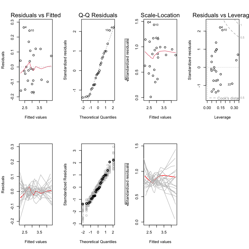
Tukey-Anscombe Plot: Residuals vs. Fitted values to check for non-linearity or heteroscedasticity.
Normal Q-Q Plot: To check the normality assumption of errors.
Scale-Location Plot: To check for constant variance.
Residuals vs. Leverage: To identify influential observations (Cook’s Distance).
Model Formulation:
Assumptions:
(normally distributed errors)
(zero expectation)
(homoscedasticity)
are stochastically independent
No perfect multicollinearity
Matrix Notation:
Gauss-Markov Theorem: Under assumptions 1-4 (without normality), OLS is BLUE (Best Linear Unbiased Estimator).
Properties:
Unbiased:
Consistent:
Asymptotic Normality:
Advanced Topics in Linear Regression Modelling
Learning Objectives
Weighted Least Squares (for non-constant variance)
Robust Fitting (to handle outliers and leverage points)
Fitting Smooth Functions (using LOESS and splines)
Additive Regression Models
Model Building strategies
Problem: OLS is not robust
Measuring Robustness
How robust an estimator is, can be investigated by two simple measures:
influence function and gross error sensitivity: The (gross error) sensitivity is based on the influence function and measures the maximum effect of a single observation on the estimated value
breakdown point: returns the minimum proportion of data that can be altered without causing completely unreliable estimates
Hence an estimator with good robustness properties has:
a bounded gross error sensitivity and
a breakdown point of (about) 0.5
Robust Regression: From OLS to MM-estimator
| Estimator | Purpose | Problem Addressed | Weights |
|---|---|---|---|
| OLS (Ordinary Least Squares) | Standard regression | None (assumes ideal conditions) | All weights = 1 |
| WLS (Weighted Least Squares) | Efficiency improvement | Heteroscedasticity (non-constant variance) | Known from variance structure |
| M-estimator (Max Likelihood) | Robustness | Outliers in response | Data-driven from residuals |
| S-estimator (Scale, ) | Robust scale | Outliers + leverage points | Implicit in scale estimation |
| MM-estimator (Modified M-estimator) | Best of both | Outliers + leverage + efficiency | Two-step: S then M |
We need S-estimators, M-estimators, and MM-estimators because real-world data often violates the assumptions of OLS regression. Therefore, we need robust estimators:
OLS has 0% breakdown point - even one bad data point can ruin your analysis
M-estimators alone can’t handle leverage points - outliers in predictors are still problematic
S-estimators are too computationally expensive for routine use
MM-estimators give us the best of both worlds - robustness AND practicality
Use MM-estimators as your default robust regression method. They provide protection against both outliers and leverage points while maintaining good statistical efficiency.
library(robustbase)
source("advanced-statistical-data-analysis/RFn_Plot-lmSim.R")
df <- read.table("advanced-statistical-data-analysis/Synthetic.dat", header=TRUE)

# Robust fit:
df.rlm <- lmrob(Y ~ x1 + x2, data=df, method="MM")

# Residual Analysis:
par(mfrow=c(2,4))
plot(df.tk.lm1)
plot.lmSim(df.tk.lm1, SEED=4711)Logistic Regression (Binary Regression)
Theoretical Background
Logistic Regression Model:
Logit Link:
Odds Ratio:
Asymptotic Properties:
Wald tests valid for large samples
df <- read.table("advanced-statistical-data-analysis/turbines.dat", header = TRUE)

# glm format: glm(x ~ y, family=…, data=…)
df.glm <- glm(cbind(Fissures, Turbines-Fissures) ~ Hours, family=binomial, data=df)
coef(df.glm)

df.p <- data.frame(Hours=seq(100, 10000, by=100))
p.y <- predict(df.glm, newdata=N, type="response")
sunflowerplot(x=df$Hours, y=df$Fissures/df$Turbines, las=1, number=df$Turbines, xlim=c(0, 10000), ylim=c(0,1))
lines(p$Hours, p.y, col=3)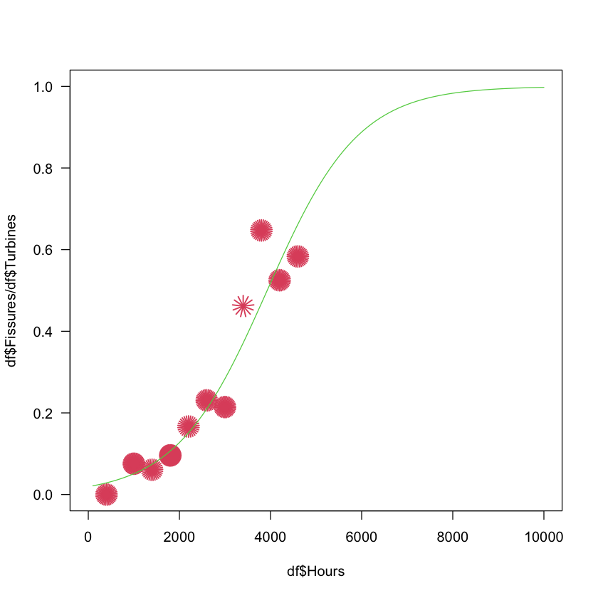
Generalized Linear Models (GLM) - A Unifying Model Family
Learning Objectives
Identify members of the exponential family
Know the two basic elements that define the GLM
Fit GLMs in R and know the algorithm underlying it
Interpret R output of a GLM fit
Exponential Family
The dispersion parameter is connected to the variance
The value is a fixed known number (weighting)
The function scales the probability to 1.
The functions and determine the distribution.
Expected Value:
where and are the first derivatives with respect to .
Variance:
Common Distributions
| Distribution | Range of | ||||||
|---|---|---|---|---|---|---|---|
| Gaussian | 1 | 1 | |||||
| Binomial | 1 | ||||||
| Poisson | 1 | 1 | |||||
| Gamma | 1 | ||||||
| Inverse Gaussian | 1 |
Distribution: The probability distribution of the response variable ;Defines the random component of the GLM
Range of : The support (set of possible values) for the response variable; Determines which distribution is appropriate for your data
: The expected value (mean) of the response; The target of your regression model
: The variance of the response variable; Determines precision of estimates
: The canonical link function from the exponential family density;
: The variance function; Connects mean to variance:
: The dispersion parameter; Scales the variance: larger means more spread
: The prior weight for each observation; Known constant for each observation (e.g., for binomial)
Normal/Gaussian:
glm(y ~ x1 + x2, family = gaussian)
# or simply: lm(y ~ x1 + x2)# Binary data
glm(y ~ x1 + x2, family = binomial)
# Aggregated data (successes and failures)
glm(cbind(success, failure) ~ x1 + x2, family = binomial)glm(y ~ x1 + x2, family = poisson)glm(y ~ x1 + x2, family = Gamma)Inverse Gaussian:
glm(y ~ x1 + x2, family = inverse.gaussian)Distribution Decision Tree
Check variance: For Poisson, verify mean ≈ variance. If variance > mean, consider Negative Binomial (not in exponential family)
Check range: Ensure response values are valid for the distribution (e.g., Poisson requires y ≥ 0)
Check skewness: Right-skewed data may need Gamma or Inverse Gaussian
Check zeros: Excess zeros may require zero-inflated models
GLM Structure
The Generalized Linear Model (GLM) is defined by two fundamental elements:
Distributional Element
The distribution of the response , given the explanatory variables , belongs to the two-parameter exponential family with:
Expectation:
Dispersion: The responses , , are independently distributed.
Structural Element
The expectation is related to the linear predictor of the explanatory variables by applying a (possibly nonlinear) function on :The function is called the link function.
The estimator for is derived based on the maximum likelihood principle:
It is defined by a nonlinear system of equations
It can be solved most efficiently by the IRLS algorithm
This two-element structure (distributional + structural) is what unifies various regression models (linear, logistic, Poisson, etc.) under the GLM framework.
IRLS Algorithm for GLM Fitting
The Iteratively Reweighted Least Squares (IRLS) algorithm fits Generalized Linear Models through the following iterative steps:
Initialize
PutEnsure Valid Weights
If necessary, modify so that the weights below are non-zero (e.g., as done by the empirical logits)Calculate Weights
Form Adjusted Response
Weighted Least Squares
Regress on by least squares to obtain . That is, solve the system of linear equations:Update Fitted Values
Calculate the fitted values:Iterate
Return to step 2 and iterate until convergence
The dispersion parameter must be estimated as well:
It can also be done by maximizing the likelihood.
As we know from multiple linear regression, we rather use an unbiased estimator for estimating the dispersion parameter
In the case of binomial and Poisson distribution:
For other distributions: see table above
Key R Code Snippets
Week 6: Inference, Model Simplification, Variable Selection
Theoretical Background
Deviance:
Deviance Test:
Overdispersion:
Confidence Intervals:
Wald:
Deviance-based: More accurate for small samples
Bootstrap: Nonparametric
Learning Objectives
Know what deviances are in GLM
Know what overdispersion is and can identify it
Know when to apply Wald-type vs deviance-based confidence intervals
Apply methods in statistical data analysis using R
Key R Code Snippets
model <- glm(y ~ x1 + x2, family = poisson, data = mydata)
null_deviance <- model$null.deviance
resid_deviance <- model$deviance
anova(model_simple, model_complex, test = "LRT")
model_poisson <- glm(y ~ x1 + x2, family = poisson, data = mydata)
dispersion <- model_poisson$deviance / model_poisson$df.residual
if (dispersion > 1.5) {
model_quasi <- glm(y ~ x1 + x2, family = quasipoisson, data = mydata)
library(MASS)
model_nb <- glm.nb(y ~ x1 + x2, data = mydata)
}AIC(model1, model2, model3)
BIC(model1, model2, model3)
step(model1, direction = "both")Week 7: Diagnostics / Model Adequacy Checking
Theoretical Background
Diagnostic Plots:
Residuals vs Fitted: Check linearity and homoscedasticity
Normal Q-Q: Check normality
Scale-Location: Check constant variance
Leverage: Identify influential points
Multicollinearity:
High VIF (> 5 or 10) indicates problematic collinearity
Effects: Unstable estimates, inflated standard errors
Learning Objectives
Understand how AIC is generalized to GLMs
Check model adequacy and determine which assumptions are violated
Find appropriate transformations of predictors in a data-driven manner
Apply methods in statistical data analysis using R
Key R Code Snippets
AIC(model1, model2)par(mfrow = c(2, 2))
plot(model_poisson, which = 1:4)
library(halfnorm)
halfnorm(residuals(model_poisson, type = "deviance"))library(car)
cooks.distance(model1)
hat.values(model1)
dfbetas(model1)Week 8: Some Extensions of GLM
Theoretical Background
Rate Models:
For Poisson with log link:
Quasi Models:
Consistent even if variance function misspecified
Standard errors adjusted by
Instrumental Variables:
First Stage:
Second Stage:
Learning Objectives
Know what a rate model is and how to analyse it with GLM
Know how a quasi model extends a GLM and when to apply it
Fit methods to data, interpret results, make inference and predictions
Key R Code Snippets
model_rate <- glm(y ~ x1 + x2, family = poisson, offset = log(t), data = mydata)model_quasipoisson <- glm(y ~ x1 + x2, family = quasipoisson, data = mydata)
model_quasibinomial <- glm(cbind(Y, m-Y) ~ x1 + x2, family = quasibinomial, data = mydata)library(AER)
model_iv <- ivreg(Y ~ X + W | Z + W, data = mydata)
summary(model_iv)Causality
Introduction
Theoretical Background
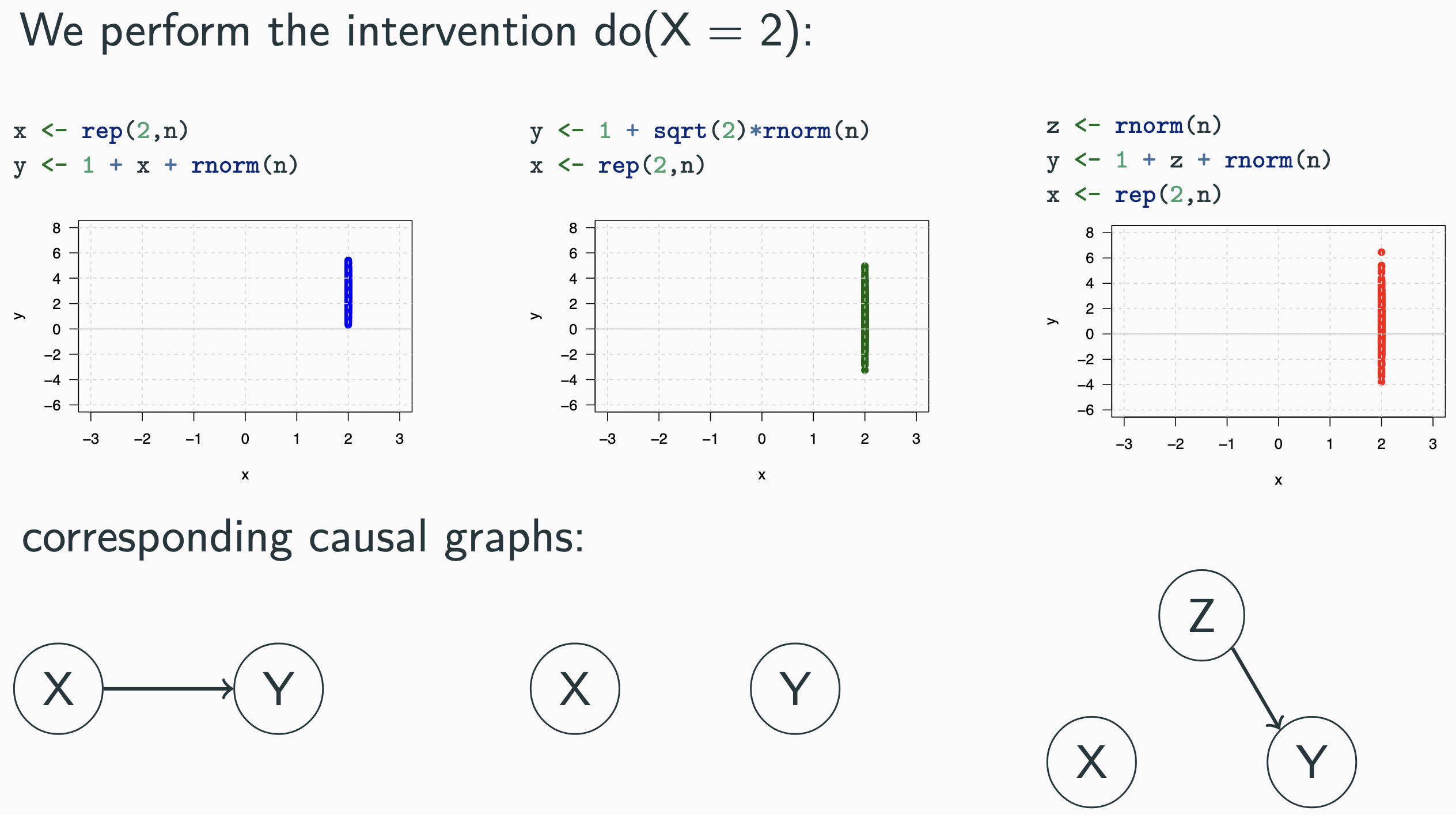
The Ladder of Causation (Pearl):
Association (Seeing): Observing patterns
Intervention (Doing): Estimating effects of actions
Counterfactuals (Imagining): Reasoning about hypotheticals
Notation:
: Conditional probability
: Causal effect
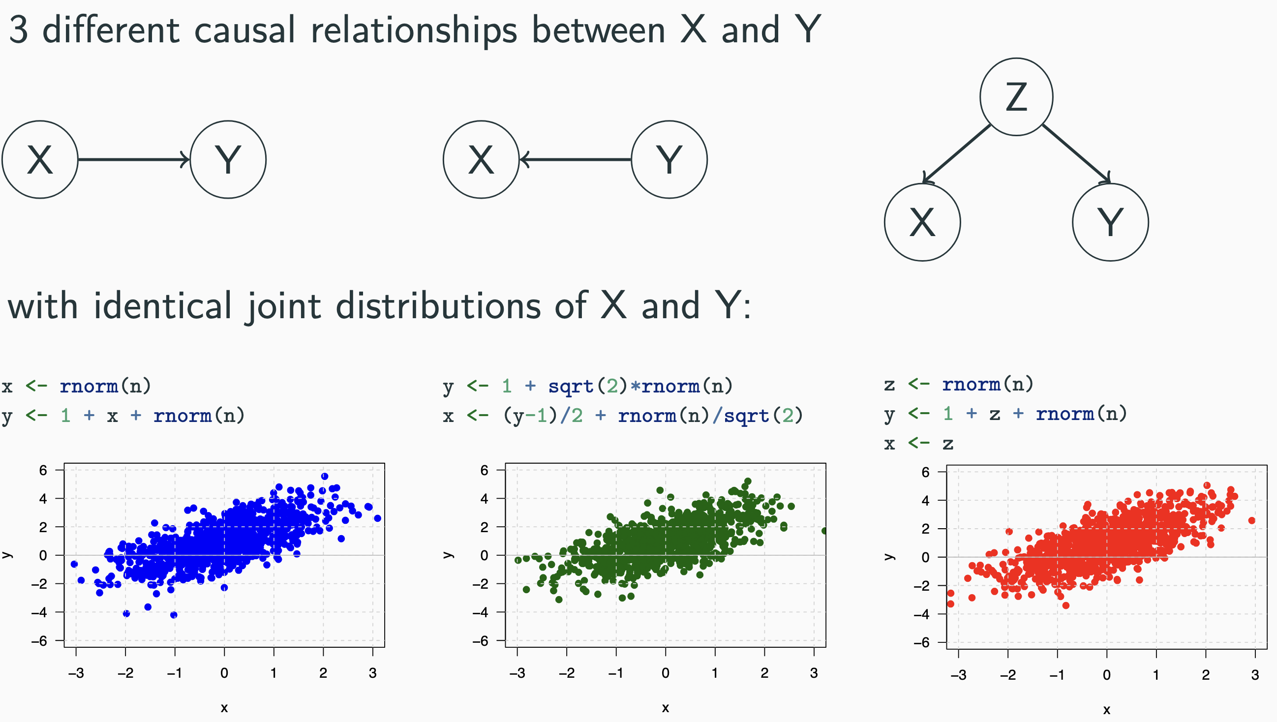
Causal Graphical Models:
Nodes: Variables
Edges: Causal relationships
DAG: Directed Acyclic Graph (no cycles)
Graphical Structures:
Chain:
and are conditionally independent given Z;
Fork:
and are conditionally independent given Z;
Collider:
and are independent , but are conditionally dependent on Z and any descendants of Z;
Learning Objectives
Understand when and why causal reasoning is important
Be familiar with causal graphical models
Understand the difference between association, interventions, and counterfactuals
Know the difference between experimental and observational data
Key R Code Snippets
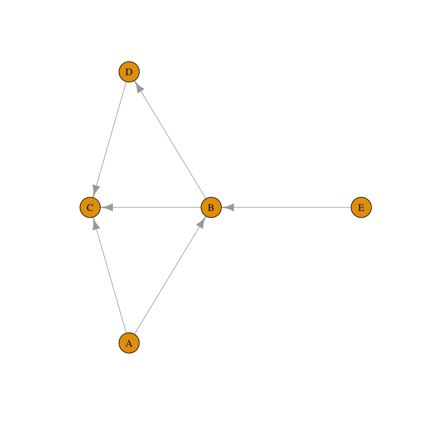
library(gRbase)
g <- dag(
c("A"),
c("B", "A", "E"), # = root node + all incoming node-edges
c("C", "A", "B", "D"),
c("D", "B"),
c("E")
)
cat("Children of B = ", children("B", g), "\n")
cat("Parents of B = ", parents("B", g), "\n")
cat("Ancestors of B = ", ancestralSet("B", g), "\n")Children of B = C D
Parents of B = A E
Ancestors of B = A B E
m <- as(g, "matrix") # to matrix from graph
m
g1 <- as(m, "igraph") # to igraph from matrix# Intervention on B (i.e. remove edges):
g2 <- removeEdge("A", "B", removeEdge("E", "B", g1))
plot(g2)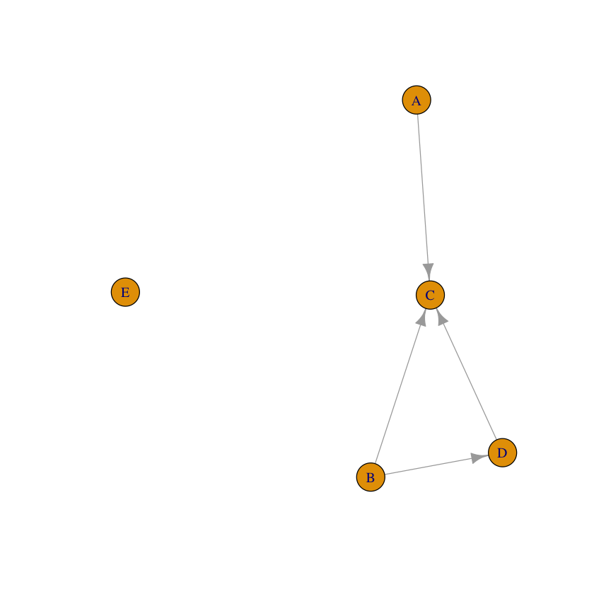
Simpson’s Paradox & Graphical Models
Theoretical Background
Simpson’s Paradox: A trend appears in different groups but disappears or reverses when combined.
Factorization:
Chain:
Fork:
Collider:
Bayesian Network Factorization:
Learning Objectives
Understand Simpson’s paradox and how to analyze it
Express joint distribution by factorization
Understand (conditional) independence
Identify (conditional) independences for chain, fork, and collider
Key R Code Snippets
library(gRbase)
library(gRain)
graph.toys <- dag(c("Gender"), c("Toy","Gender"))
load("advanced-statistical-data-analysis/toys.rda")
gn <- grain(graph.toys, data = toys) # combine graph and data to a Bayesian network# Conditional probability: from data
toys_girls <- toys[toys$Gender== "girl",]
cat("P(Toy = car | Gender = girl) =", sum(toys_girls== "car") / nrow(toys_girls))
# Conditional probability: from the Bayesian network
querygrain(gn, nodes=c("Toy", "Gender"), type="conditional")P(Toy = car | Gender = girl) = 0.3915344# Joint probability: from data
n_car_girl <- sum(toys$Toy== "car" & toys$Gender== "girl")
cat("P(Toy = car, Gender = girl) =", n_car_girl/nrow(toys))
# Joint probability: from the Bayesian network
querygrain(gn, nodes=c("Toy", "Gender"), type="joint")P(Toy = car, Gender = girl) = 0.1749409# marginal probabilities
querygrain(gn, nodes = "Gender", type = "marginal")
querygrain(gn, nodes = "Toy", type = "marginal")# Manually using a Conditional Probability Table:
gender <- cptable("Gender", values = c(0.55, 0.45), levels = c("boy","girl"))
toy <- cptable("Toy", values = c(0.67, 0.33), levels = c("car","doll"))
toy_gender <- cptable(c("Toy", "Gender"),
# car:boy = 0.89, doll:boy = 0.10, car:girl = 0.39, doll:girl = 0.60
values = c(0.89, 0.10, 0.39, 0.60), levels = c("car","doll"))
# Building the Bayesian Network
cpt <- compileCPT(list(gender, toy_gender))
bn <- grain(cpt, compile = FALSE)
plot(bn)
querygrain(bn, nodes=c("Toy", "Gender"), type="conditional")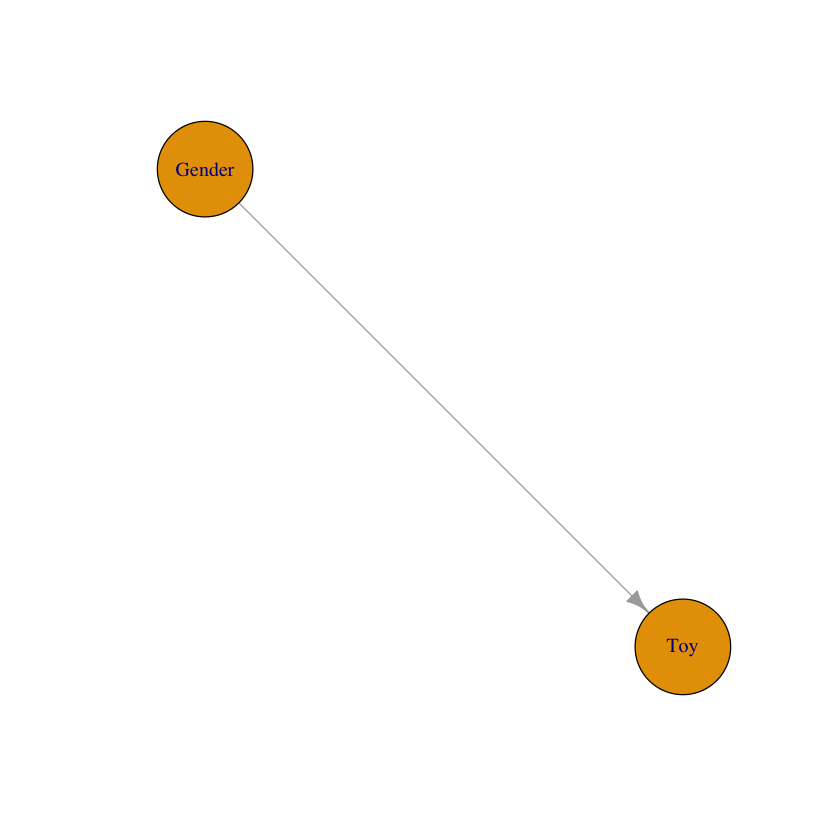
D-Separation & Causal Effect Estimation
Theoretical Background
D-Separation:
X and Y are d-separated given Z if all paths between X and Y are blocked by Z if and only if:
a middle node of a chain (X → B → Y) or a fork (X ← B → Y) is conditioned on (i.e. it is in Z)
a middle node of a collider (X → B ← Y) is not conditioned on (i.e. is not in Z), and no descendant of B is in Z.
If Z blocks every path between two nodes X and Y, then X and Y are d-separated conditioning on Z and thus are conditionally independent on Z.
Adjustment Formula:
Backdoor Criterion: Z satisfies backdoor criterion if:
Z blocks all backdoor paths from X to Y
Z does not contain any descendants of X
Learning Objectives
Know D-Separation
Estimate causal effect using the adjustment formula
Define adjustment sets with the backdoor criterion
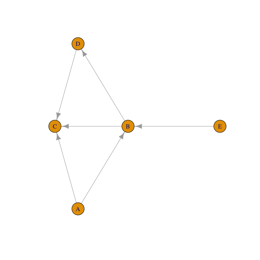
library(gRbase)
# List all nodes with their parents
g <- dag("A",c("B","A","E"),c("C","A","B","D"),c("D","B"),c("E"))
d.separates <- function(a,b,c,dag){
separates(a,b,c, moralize(ancestralGraph(union(union(a,b),c),dag)))
}
plot(g)
cat("Are E and D d-separated by Z = {B}?", d.separates("E", "D", c("B"), g), "\n")
cat("Are E and C d-separated by Z = {A}?", d.separates("E", "C", c("A"), g), "\n")
cat("Are A and D d-separated by Z = {B, C}?", d.separates("A", "D", c("B", "C"), g), "\n")Are E and D d-separated by Z = {B}? TRUE
Are E and C d-separated by Z = {A}? FALSE
Are A and D d-separated by Z = {B, C}? FALSE
Structural Causal Models
Theoretical Background
Linear SCM:
Direct vs. Total Effects:
Total: Effect through all paths
Direct: Effect through direct path only
Learning Objectives
Be familiar with (linear) structural causal models
Understand direct and total causal effects
Estimate direct and total causal effect from linear SCM
Key R Code Snippets
library(gRbase)
library(igraph)
set.seed(253)
g <- dag(
c("Study", "Teacher", "Prior", "Attendance"),
c("Attendance", "Prior", "Teacher"),
c("Exam", "Study", "Prior")
)
E(g)$weight <- c(-5, -3, -3, -2, 4, 8, 3)
plot(g, edge.label = E(g)$weight)
n <- 1000000 # Sample size
# Simulate data from the SCM (using the DAG's coefficients)
prior <- rnorm(n)
teacher <- rnorm(n)
attendance <- -2 * prior + 4 * teacher + rnorm(n)
study <- -3 * prior - 5 * teacher + -3 * attendance + rnorm(n)
exam <- 3 * prior + 8 * study + rnorm(n)
# Estimate total causal effect of attendance on exam
fit <- lm(exam ~ attendance + prior + teacher)
coef(fit)["attendance"] # Returns the estimated effect (-24 for large n)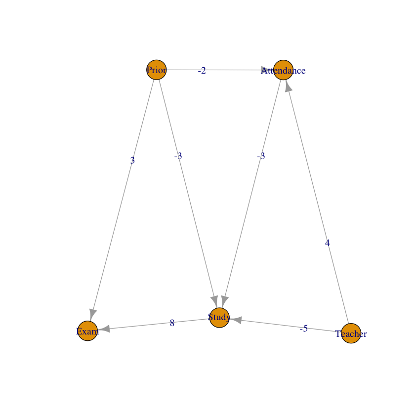
Advanced Topics
Theoretical Background
Instrumental Variables:
Relevance:
Exclusion: Z has no direct effect on Y except through X
Exogeneity:
Two-Stage Least Squares:
First stage:
Second stage:
Counterfactuals: Pearl’s three-step method:
Abduction: Use the observed information to determine the values of the noise variables.
Action: Modify the causal model M by removing the structural equation for the variable X and replacing with X = x.
Prediction: Use the modified model to compute the counterfactual.
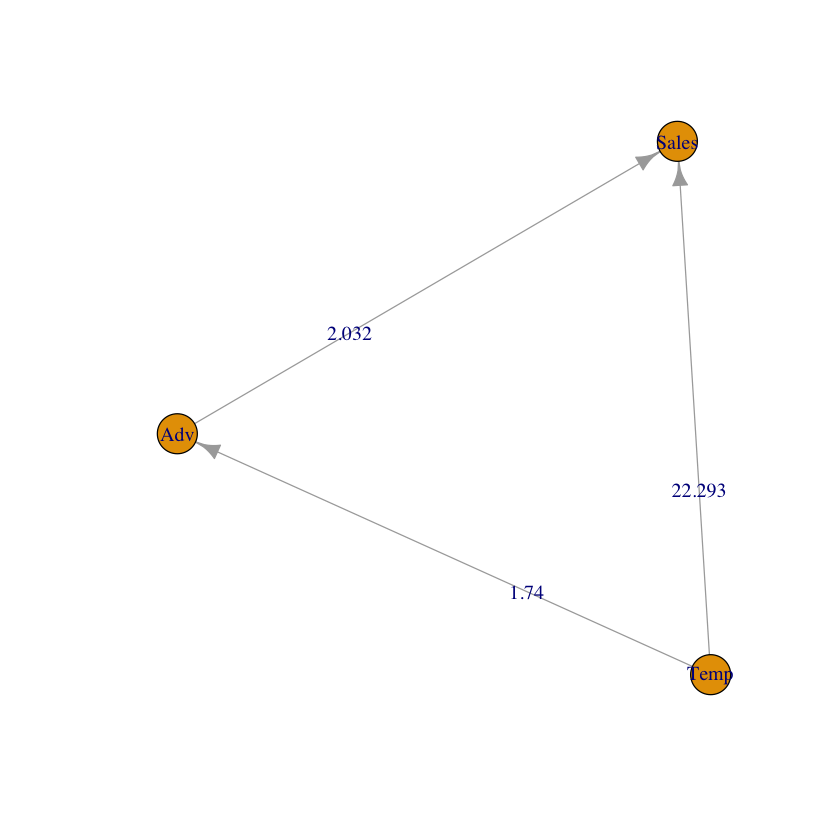
library(gRain)
g <- dag(
c("Temp"),
c("Adv", "Temp"),
c("Sales", "Temp", "Adv")
)
load("advanced-statistical-data-analysis/ice_cream.rda")
lm.adv <- lm(Adv ~ Temp, data = ice_cream)
lm.sales <- lm(Sales ~ Temp + Adv, data = ice_cream)
print(lm.adv)
print(lm.sales)
E(g)$weight <- c(1.74, 22.293, 2.032)
plot(g, edge.label = E(g)$weight)
# look at the observation with the highest daily temperature:
ice_cream[ice_cream$Temp == max(ice_cream$Temp), ]
day19 <- ice_cream[19,]
# Counterfactuals:
# 1. Abduction:
Es <- day19$Sales - (22.293 * day19$Temp + 2.032 * day19$Adv)
Ea <- day19$Adv - (1.74 * day19$Temp)
Et <- day19$Temp
# how many ice creams would have been sold on that day, if
# temperature would have been 30? -> do(Temp = 30):
# 2. Action:
temp_c1 <- 30
adv_c1 <- 1.74 * temp_c1 + Ea
# 3. Prediction:
sales_c1 <- 22.293 * temp_c1 + 2.032 * adv_c1 + Es
cat("if the temperature would have been", temp_c1, "then", sales_c1, "ice creams would have been sold", "\n")
# do(Adv = 0):
# how many ice creams would have been sold on that day, if
# there would have been no advertisement? -> do(Adv = 0):
# 2. Action:
temp_c2 <- day19$Temp
adv_c2 <- 0
# 3. Prediction:
sales_c2 <- 22.293 * temp_c2 + 2.032 * adv_c2 + Es
cat("without advertisement on that day,", sales_c2, "ice creams would have been sold", "\n")
# Use linear regression to predict the average number of ice creams sold for the counterfactuals
x0 <- data.frame(
Temp = c(30, day19$Temp),
Adv = c(day19$Adv, 0))
cat("Average number of ice creams sold for days with given temperature and advertisement: ", predict(lm.sales, newdata = x0), "\n")
# The prediction describes the average number of ice creams. In contrast,
# the counterfactual describes how many ice creams would have been sold on the
# specific day (corresponding to data point 19) if the temperature
# and advertising had been different.
Call:
lm(formula = Adv ~ Temp, data = ice_cream)
Coefficients:
(Intercept) Temp
110.94 1.74
Call:
lm(formula = Sales ~ Temp + Adv, data = ice_cream)
Coefficients:
(Intercept) Temp Adv
-258.252 22.293 2.032
if the temperature would have been 30 then 779.1024 ice creams would have been sold
without advertisement on that day, 530.5143 ice creams would have been sold
Average number of ice creams sold for days with given temperature and advertisement: 764.971 501.93
Markov Equivalence:
Chains and Forks are Markov equivalent, i.e. their graphs imply the same conditional independencies.
Colliders encode a different independence.
→ Colliders are identifiable from data, whereas fork and chains are not
→ All graphs where we can flip the arrows without introducing new colliders and keeping all existing colliders are Markow Equivalent.
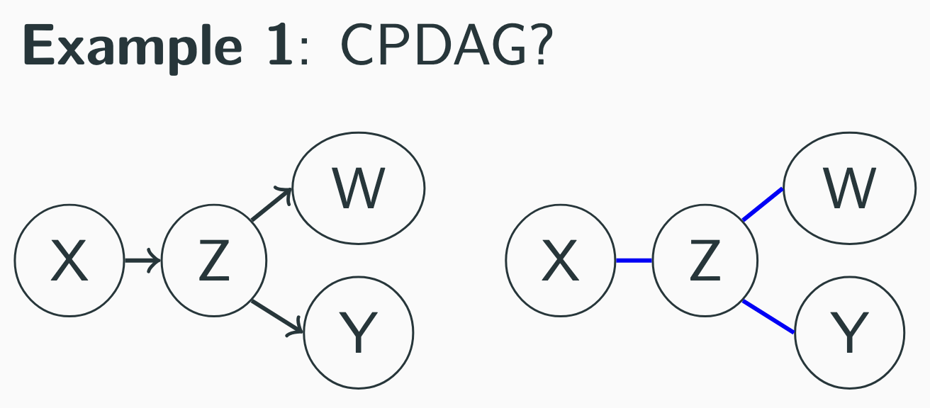
Markov Equivalence can be represented by a CPDAG.
Completed Partially DAG (CPDAG)
represents the Markov equivalence class of DAGs
Directed edge: causal direction is clear (all graphs agree)
Undirected edge: causal direction is ambiguous (graphs disagree)
Encodes what can be identified from data alone
Learning Objectives
Understand instrumental variables
Be familiar with counterfactual reasoning
Know the three steps in computing counterfactuals
Understand Markov Equivalence
Key R Code Snippets
library(AER)
model_iv <- ivreg(Y ~ X + W | Z + W, data = mydata)
summary(model_iv)
first_stage <- lm(X ~ Z + W, data = mydata)
summary(first_stage)library(pcalg)
dag1 <- dag(c("X", "Z", "Y"), list(c("X", "Z"), c("Z", "Y")))
dag2 <- dag(c("X", "Z", "Y"), list(c("Z", "X"), c("Z", "Y")))
meq(dag1, dag2)Causal Structure Learning
Theoretical Background
Assumptions of Independence-Based Methods:
Causal sufficiency, i.e., no unobserved confounding variables.
Acyclicity: No directed cycles in the graph
Markov: Graph → Data, i.e., if X and Y are d-separated by Z in the graph, then X and Y are conditionally independent given Z.
Faithfulness: Data → Graph, i.e., if X and Y are conditionally independent given Z, then X and Y are d-separated by Z in the graph.
What about non-Gaussian structural equations? LinGAM to the rescue!
4 Steps of Causal Inference
DAG: Create a causal model using expert knowledge.
Identification: Determine whether and how the causal effect can be identified from the observational data.
Estimation: Estimate the causal effect from the data.
Validity: Test the estimated causal effect:
| Method | Idea | Good if ... |
|---|---|---|
| Random Cause | Add random covariate | Estimate stable |
| Placebo | Randomize treatment X | Estimate |
| Data Subset | cross-validation / bootstrap | Estimates similar |
Key R Code Snippets
# PC Algorithm:
library(pcalg)

# Example data generation
set.seed(239)
N <- 500000
X <- rnorm(N)
Z <- rnorm(N)
W <- 5 * X + 10 * Z + rnorm(N)
Y <- 12 * W + rnorm(N)
V <- 8 * W + rnorm(N)
dat <- cbind(X, Z, W, Y, V)

suffStat <- list(C = cor(dat), n = nrow(dat))
pc.fit <- pc(
    suffStat,
    indepTest = gaussCItest,
    alpha = 0.01,
    labels = colnames(dat),
    verbose = FALSE)
summary(pc.fit)  # There are 19 + 29 + 12 + 4 tests!!
plot(pc.fit, main = "") # Needs a title!
Object of class 'pcAlgo', from Call:
pc(suffStat = suffStat, indepTest = gaussCItest, alpha = 0.01,
labels = colnames(dat), verbose = FALSE)
Nmb. edgetests during skeleton estimation:
===========================================
Max. order of algorithm: 3
Number of edgetests from m = 0 up to m = 3 : 19 29 12 4
Graphical properties of skeleton:
=================================
Max. number of neighbours: 2 at node(s) 3
Avg. number of neighbours: 0.8
Adjacency Matrix G:
X Z W Y V
X . . 1 . .
Z . . 1 . .
W . . . 1 1
Y . . . . .
V . . . . .

# LiNGAM Algorithm:
library(pcalg)

# Linear SCM with uniform distributed noise
set.seed(145)
N <- 2000
x1 <- runif(N,-.5,.5)
x2 <- runif(N,-.3,3)
x3 <- x1 + x2 + runif(N,-.7,.7)
x4 <- 2*x1 + runif(N,-.5,.5)
x5 <- 3*x3 + runif(N,-1,1)
data <- cbind(x1,x2,x3,x4,x5)

# Apply LiNGAM
fit.ex2 <- lingam(data)

# Transpose the matrix to correct edge directions
adj_matrix <- t(fit.ex2$Bpruned)

# Convert to igraph and plot
g <- graph_from_adjacency_matrix(
  adj_matrix,
  mode = "directed",
  weighted = TRUE
)
plot(g, edge.label = round(E(g)$weight, 2))  # Show rounded weights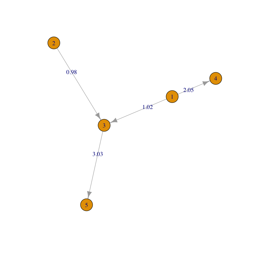
Modified logit transformation to avoid divison by zero for full range of percentage (0-100%). Unmodified: