Bayesian Machine Learning
Philosophical Foundations and Bayes’ Theorem
Interpretations of probability
Frequentist definition: Probability of event is the long-run relative frequency of in infinitely many repetitions of the same experiment. Statements are about data, not parameters ( is defined via an idealized limit of repetitions).
Bayesian definition: Probability is a subjective degree of belief about events or parameters, given current knowledge ( quantifies how plausible you think is).
Key philosophical contrast
Frequentist: uncertainty is in the world (randomness of experiments).
Bayesian: uncertainty is in the head of the observer (state of information; different observers with different prior knowledge can have different probabilities).
Sampling vs. inference
Sampling (forward problem): Assume parameter is known, ask: “If is the probability of success, what is ?”. For example: Number of heads in 10 tosses with known ~ Binomial().
Inference (inverse problem): Assume data is observed, but the parameters are unknown, ask: “Given I observed heads in 10 tosses, what do I believe about ?”
Frequentist: Estimate single “best” value (e.g. MLE )
Bayesian: derive a posterior distribution over :
Bayes’ theorem and roles of likelihood
Bayes’ theorem (discrete):
Belief-updater view:
Prior: beliefs before data.
Likelihood: how plausible data are under different parameter values.
Posterior: updated beliefs after data.
Likelihood in both schools:
In frequentist statistics, the likelihood function is used to perform Maximum Likelihood Estimation (MLE). This identifies the single parameter value that maximizes the probability of having produced the observed data.
In Bayesian statistics, the likelihood function serves as a belief updater. It is multiplied by the prior distribution to calculate the posterior, allowing you to estimate a full distribution of all plausible values rather than just one “best” number.
When Bayesian methods are preferable
Small sample sizes / rare events: frequentist asymptotics unreliable.
Strong prior information available (expert opinion, previous studies) and should be integrated.
Need full uncertainty quantification (posterior distributions, credible intervals) rather than point estimates or p-values.
Complex hierarchical or graphical models, where likelihood-based methods get complicated but Bayesian methods remain conceptually coherent.
The computational curse of Bayesian statistics
Core difficulty: the evidence (marginal likelihood) is an often intractable integral:
In simple conjugate families this integral is analytic.
In realistic models (many parameters, non-Gaussian likelihoods), high‑dimensional integrals are impossible to compute in closed form.
This computational curse motivates Markov Chain Monte Carlo (MCMC) and Variational Inference.
Conjugate Families and Continuous Inference
Conjugate families are pedagogically useful to understand how priors and data trade off.
Beta-Binomial
Likelihood:
is the binomial coefficient, representing the number of ways to choose successes from trials:
is the probability of getting exactly successes
is the probability of getting exactly failures
Prior:
with:
Posterior:
Key properties: Prior “pseudo-counts”: successes, failures
With more data, likelihood dominates; with little data, prior dominates
Order of data does not matter; only sufficient statistics
Notebook Cell
import numpy as np
import matplotlib.pyplot as plt
from scipy import stats

def plot_beta_binomial( alpha, beta, n, k, figsize=(13,3) ):
    # create figure
    plt.figure( figsize=figsize )

    # numeric evaluation range for pi
    pi_range = np.linspace(0, 1, 1000)

    # prior
    prior = [stats.beta.pdf(pi, a=alpha, b=beta) for pi in pi_range]
    plt.plot( pi_range, prior, alpha=0.5, label="prior", c="orange" )
    plt.fill_between( pi_range, prior, alpha=0.3, color="orange" )

    # scaled likelihood
    likelihood = [stats.binom.pmf(n=n, k=k, p=pi) for pi in pi_range]
    likelihood /= np.sum( likelihood ) * (pi_range[1]-pi_range[0])
    plt.plot( pi_range, likelihood, alpha=0.5, label="(scaled) likelihood", c="blue" )
    plt.fill_between( pi_range, likelihood, alpha=0.3, color="blue" )

    # posterior
    posterior = [stats.beta.pdf(pi, a=alpha+k, b=beta+n-k) for pi in pi_range]
    plt.plot( pi_range, posterior, alpha=0.5, label="posterior", color="darkgreen" )
    plt.fill_between( pi_range, posterior, alpha=0.3, color="darkgreen" )

    # enable legend and set descriptive title
    plt.legend( fontsize=14 )
    plt.title( "$\\alpha = {}, \\beta={}, n={}, k={}$".format(alpha, beta, n, k) )

plot_beta_binomial(alpha=5, beta=11, n=20, k=9)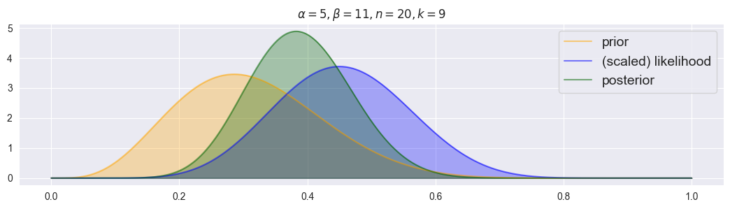
Notebook Cell
# Likelihood (Binomial counts):
import preliz as pz
pz.Binomial(n=1, p=0.75).plot_pdf()
<Axes: >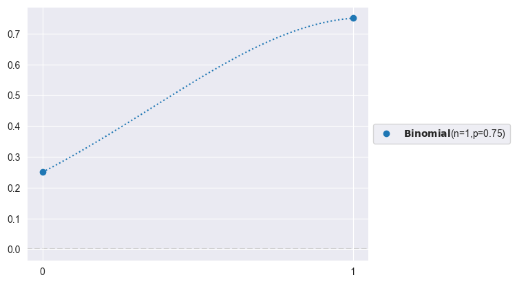
Notebook Cell
# Prior:
import preliz as pz
pz.Beta(alpha=3, beta=5).plot_pdf()
<Axes: >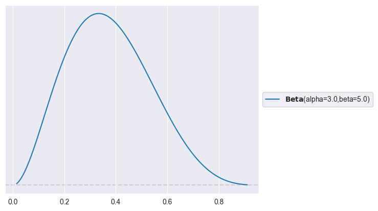
Poisson–Gamma: For Counts
Likelihood:
is the contribution from events occurring
is the probability of no other events occurring
normalizes for the ordering of events
Prior:
with
Posterior:
Key properties: Prior “pseudo-counts”: represents prior event count, represents prior observation periods.
With more data, likelihood dominates; with little data, prior dominates.
Order of data does not matter; only sufficient statistic .
Notebook Cell
def plot_gamma_poisson(alpha, beta, y, figsize=(13, 3)):
    y = np.asarray(y)
    n = len(y)
    sum_y = y.sum()

    # Posterior hyperparameters
    alpha_post = alpha + sum_y
    beta_post  = beta + n

    # Choose a range for lambda using high quantiles of prior and posterior
    # (robust and adaptive to parameter scale)
    # scipy.stats.gamma uses shape 'a' and scale = 1/rate
    scale_prior = 1.0 / beta
    scale_post  = 1.0 / beta_post

    lam_max = max(
        stats.gamma.ppf(0.999, a=alpha,      scale=scale_prior),
        stats.gamma.ppf(0.999, a=alpha_post, scale=scale_post)
    )
    lam_range = np.linspace(0, lam_max, 1000)

    plt.figure(figsize=figsize)

    # Prior
    prior = stats.gamma.pdf(lam_range, a=alpha, scale=scale_prior)
    plt.plot(lam_range, prior, alpha=0.5, label="prior", c="orange")
    plt.fill_between(lam_range, prior, alpha=0.3, color="orange")

    # Likelihood as function of lambda: L(λ) = ∏_i Pois(y_i | λ)
    # Use log-likelihood for numerical stability
    log_like = np.zeros_like(lam_range)
    for yi in y:
        log_like += stats.poisson.logpmf(yi, mu=lam_range)
    likelihood = np.exp(log_like)

    # Numerically normalize likelihood over lam_range so it behaves like a pdf on this grid
    norm_const = np.trapz(likelihood, lam_range)
    if norm_const > 0:
        likelihood /= norm_const
    plt.plot(lam_range, likelihood, alpha=0.5, label="(scaled) likelihood", c="blue")
    plt.fill_between(lam_range, likelihood, alpha=0.3, color="blue")

    # Posterior
    posterior = stats.gamma.pdf(lam_range, a=alpha_post, scale=scale_post)
    plt.plot(lam_range, posterior, alpha=0.5, label="posterior", color="darkgreen")
    plt.fill_between(lam_range, posterior, alpha=0.3, color="darkgreen")

    # Legend and title
    plt.legend(fontsize=14)
    plt.xlabel(r"$\lambda$")
    plt.title(r"$\alpha = {}, \beta = {}, n = {}, \sum y_i = {}$"
              .format(alpha, beta, n, int(sum_y)))
    plt.tight_layout()
    plt.show()

plot_gamma_poisson(alpha=2.0, beta=0.75, y=[7, 8, 3, 7, 11, 7, 9, 19, 7, 15, 9, 5, 12, 3, 7, 6, 5, 3, 11, 5])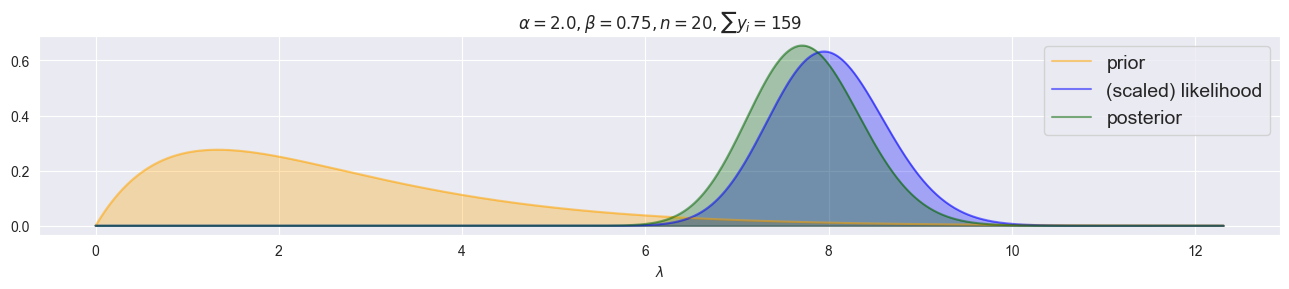
Negative Binomial For Overdispersed Counts
Unlike the Poisson distribution, the variance is not equal to the mean; it is larger (overdispersion). As the dispersion parameter , the Negative Binomial distribution converges to the Poisson distribution. The Negative Binomial likelihood does not have a simple closed-form conjugate posterior - posterior inference must be done via MCMC simulation.
Likelihood:
probability of success
is the number of successes (-1 because last success is fixed as its the stopping criterion)
is the number of failures
Prior: Negative Binomial is typically used in models where conjugacy does not hold. Therefore, we often use:
in simple models or in regression with
or (must be positive)
Normal–Normal (variance needs to be known!)
Likelihood:
is the mean (location parameter)
is the variance (assumed known)
measures squared deviation from the mean
Prior:
is the prior mean
is the prior variance (reflects uncertainty about )
Posterior:
Key properties: Posterior mean is a precision-weighted average of prior mean and data .
Precision = : higher precision = more influence.
Posterior variance is always smaller than both prior and data variance (information accumulation).
With more data ( observations), data precision dominates.
Notebook Cell
def plot_normal_normal(mu0, tau0, sigma, y, figsize=(13, 3)):
    y = np.asarray(y)
    n = len(y)
    ybar = y.mean()

    # Posterior variance and mean
    tau_n2 = 1.0 / (n / sigma**2 + 1.0 / tau0**2)
    mu_n = tau_n2 * (n * ybar / sigma**2 + mu0 / tau0**2)
    tau_n = np.sqrt(tau_n2)

    # Choose a plotting range for mu around data and prior
    mu_min = min(ybar - 4 * sigma, mu0 - 4 * tau0, mu_n - 4 * tau_n)
    mu_max = max(ybar + 4 * sigma, mu0 + 4 * tau0, mu_n + 4 * tau_n)
    mu_range = np.linspace(mu_min, mu_max, 1000)

    plt.figure(figsize=figsize)

    # Prior over mu
    prior = stats.norm.pdf(mu_range, loc=mu0, scale=tau0)
    plt.plot(mu_range, prior, alpha=0.5, label="prior", c="orange")
    plt.fill_between(mu_range, prior, alpha=0.3, color="orange")

    # Likelihood as function of mu (up to constant)
    # Equivalent to N(mu | ybar, sigma^2/n)
    like_unnorm = stats.norm.pdf(mu_range, loc=ybar, scale=sigma / np.sqrt(n))
    # Numerically normalize to integrate ~1 on this grid
    norm_const = np.trapz(like_unnorm, mu_range)
    likelihood = like_unnorm / norm_const if norm_const > 0 else like_unnorm

    plt.plot(mu_range, likelihood, alpha=0.5, label="(scaled) likelihood", c="blue")
    plt.fill_between(mu_range, likelihood, alpha=0.3, color="blue")

    # Posterior over mu
    posterior = stats.norm.pdf(mu_range, loc=mu_n, scale=tau_n)
    plt.plot(mu_range, posterior, alpha=0.5, label="posterior", color="darkgreen")
    plt.fill_between(mu_range, posterior, alpha=0.3, color="darkgreen")

    # Legend and title
    plt.legend(fontsize=14)
    plt.xlabel(r"$\mu$")
    plt.title(
        r"$\mu_0 = {:.2f}, \tau_0 = {:.2f}, \sigma = {:.2f}, n = {}, \bar y = {:.2f}$"
        .format(mu0, tau0, sigma, n, ybar)
    )
    plt.tight_layout()
    plt.show()

np.random.seed(0)
plot_normal_normal(mu0=0.0, tau0=1.0, sigma=2.0, y=np.random.normal(loc=5.0, scale=2.0, size=10))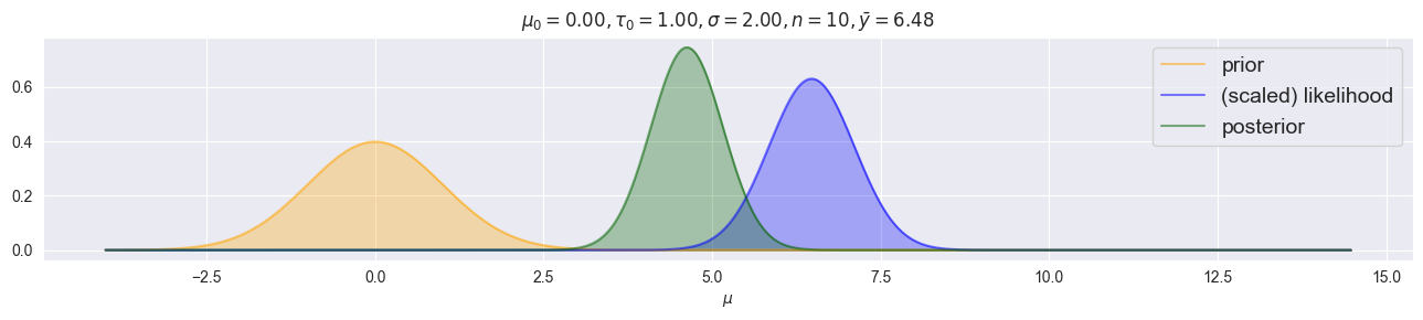
Multivariate Problems
Covariance: Quantifying Relationship Between Variables
: A variable’s covariance with itself is its variance
: and are unrelated; on average there is no “co-variance”
For observed data (empirical), the sample covariance is:
and : the sample means
is the number of observations (the denominator is to account for the loss of one degree of freedom when estimating the means)
Pearson Correlation = Standardized Covariance
Pearson correlation normalizes covariance by the standard deviations of both variables, producing a unitless measure bounded between 0 and 1. By standardizing covariance, correlation becomes interpretable on a common scale where indicates perfect positive correlation, indicates no correlation, and indicates perfect negative correlation.
and are the standard deviations of and respectively
For observed data (empirical), the Pearson Correlation is:
and are the sample standard deviations
Multinomial–Dirichlet: For Categorical Counts (Generalized Beta-Binomial)
Use whenever we want to model experiments with > 2 mutually exclusive outcomes!
Likelihood:
is the contribution from observed category counts
normalizes for the number of orderings
Constraint: and
Prior:
with
Posterior:
Key properties: Prior “pseudo-counts”: represents prior observations in category . Setting (flat prior) means no prior preference.
With more data, likelihood dominates; with little data, prior dominates.
Order of data does not matter; only sufficient statistic .
Conjugate family ensures posterior is also Dirichlet with simple parameter update.
Multivariate Normal
, with mean and covariance matrix
Closed under linear transformations, addition, marginalization, conditioning
Covariance controls scale and correlation; must be symmetric and positive definite
LKJ prior for correlation matrices: flexible prior on correlation structures; together with priors on standard deviations gives LKJCov prior for
Multinomial–Dirichlet
Likelihood: counts over categories, .
Prior: Dirichlet, .
Posterior: Dirichlet, where counts in category .
Used for compositional data (election results, topic proportions).
Markov Chain Monte Carlo and the Metropolis Algorithm
Goal: obtain samples from when no closed form is available. MCMC constructs a Markov chain whose stationary distribution is the posterior.
Metropolis algorithm (random-walk variant)
Notebook Cell
from scipy import stats
import seaborn as sns
from tqdm.auto import tqdm
import matplotlib.pyplot as plt
def propose_jump(pi, sigma):
return stats.norm.rvs( loc=pi, scale=sigma )
def decide(pi, pi2, alpha, beta, n, k, debug=False):
# evaluate prior and likelihood
prior1 = stats.beta.pdf( pi, alpha, beta )
prior2 = stats.beta.pdf( pi2, alpha, beta )
likelihood1 = stats.binom.pmf( n=n, k=k, p=pi )
likelihood2 = stats.binom.pmf( n=n, k=k, p=pi2 )
# define alpha
alpha = min(1, prior2/prior1 * likelihood2/likelihood1)
if debug: print("pi = {:.5f}, pi2 = {:.5f}, alpha = {:.5f}".format(pi, pi2, alpha))
# jump decision
p = np.random.rand()
if p<=alpha and 0 < pi2 < 1:
return pi2
else:
return pi
def metropolis_chain(n_steps, alpha, beta, n, k, sigma):
# initialize
pi = np.random.rand()
chain = []
# create chain
for i in tqdm( range( n_steps ) ):
pi2 = propose_jump( pi, sigma )
pi = decide( pi, pi2, alpha, beta, n, k )
chain.append( pi )
return chain
def metropolis( n_chains, n_steps, alpha, beta, n, k, sigma ):
res = [metropolis_chain( n_steps, alpha, beta, n, k, sigma ) for i in range( n_chains)]
return np.array(res).T # to have chains in columns
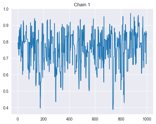
def trace_plots(sim):
for i in range( sim.shape[1] ):
plt.figure()
plt.plot( sim[:,i] )
plt.title("Chain {}".format(i+1))
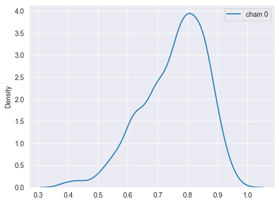
def density_plots( sim ):
plt.figure()
for i in range( sim.shape[1] ):
sns.kdeplot( sim[:,i], label="chain {}".format(i) )
plt.legend()
def rhat( sim ):
total_var = np.var( sim.flatten() )
individual_var = np.var( sim, axis=0 )
rhat = np.sqrt( total_var / np.mean(individual_var) )
return rhat
sim = metropolis(n_chains=1, n_steps=1000, alpha=5, beta=2, n=10, k=8, sigma=0.2)
trace_plots(sim)
density_plots(sim)
print(f"Rhat: {rhat(sim)}")Rhat: 1.0
For target density and symmetric proposal distribution , the Metropolis steps are:
Initialize (e.g. some reasonable value).
For iterations :
Propose new state . E.g. random walk: .
Compute acceptance probability
Accept or reject: Draw , If , set (move), Else set (stay).
After burn‑in and thinning, use remaining samples as approximate draws from the posterior.
Proposal distribution: the distribution from which proposed new parameters are drawn (). Choice of its scale strongly affects mixing and acceptance rate.
MCMC with PyMC
import pymc as pm
# PyMC for Beta-Binominal Conjugate Family
with pm.Model() as beta_binom_model:
    pi = pm.Beta("pi", alpha=5, beta=2)
    y = pm.Binomial("y", p=pi, n=10, observed=8)
    trace = pm.sample(1000)
Output
Notebook Cell
import arviz as az
import pandas as pd

def uncertainty_binominal(trace_posterior, var_name: str, n: int, **kwargs):
    assert var_name != None, "var_name is required for pi"
    assert n != None and n > 0, "n must be > 0"

    values = trace_posterior[var_name].values
    aleatoric_var = (n * values * (1.0 - values)).mean()
    epistemic_var = (values * n).var(ddof=1)

    return aleatoric_var, epistemic_var

def uncertainty_normal(trace_posterior, mu: str = "mu", sigma: str = "sigma", **kwargs):
    aleatoric_var = (trace_posterior[sigma].values**2).mean()
    epistemic_var = trace_posterior[mu].var(ddof=1).values

    return aleatoric_var, epistemic_var

def uncertainty_poisson(trace_posterior, var_name: str, n: int, **kwargs):
    assert var_name != None, "var_name is required for lambda"

    values = trace_posterior[var_name].values
    aleatoric_var = values.mean()
    epistemic_var = values.var(ddof=1)

    return aleatoric_var, epistemic_var

def uncertainty_summary(trace_posterior, family=None, **kwargs):
    """
    Computes the aleatoric (data), epistemic (model uncertainty) and predictive (overall uncertainty) variance of a pymc trace.posterior

    Parameters
    ----------
    trace_posterior : array_like
        Array containing numbers whose mean is desired. If `a` is not an
        array, a conversion is attempted.
    family : str
        Either one of 'binominal', 'normal' or 'poisson'.

    For family='binominal':
    -----------------------
    var_name : str
        Name of the Pi variable in the trace_posterior
    n : int
        Number of trials

    For family='normal':
    -----------------------
    mu : str
        Name of the parameter that represents the mean of the normal distribution.

    sigma : str
        Name of the parameter that represents the standard deviation of the normal distribution.

    For family='poisson':
    -----------------------
    var_name : str
        Name of the lambda variable in the trace_posterior
    """
    assert trace_posterior != None, "trace_posterior must be provided"
    assert family != None, "family must be provided"

    uncertainty_stats = pd.DataFrame()
    match family:
        case 'binominal':
            aleatoric_var, epistemic_var = uncertainty_binominal(trace_posterior, **kwargs)
        case 'normal':
            aleatoric_var, epistemic_var = uncertainty_normal(trace_posterior, **kwargs)
        case 'poisson':
            aleatoric_var, epistemic_var = uncertainty_poisson(trace_posterior, **kwargs)
        case _:
            raise ValueError(f"Unknown family: {family}")

    predictive_var = aleatoric_var + epistemic_var

    uncertainty_stats[family] = {
        'var_aleatoric': aleatoric_var,
        'var_epistemic': epistemic_var,
        'var_predictive': predictive_var,
        'var_aleatoric_percent': aleatoric_var / predictive_var,
        'var_epistemic_percent': epistemic_var / predictive_var,
    }

    # switch rows and columns:
    uncertainty_stats = uncertainty_stats.T

    return uncertainty_stats

def trace_summary(trace, hdi_prob=0.8, var_names=None):
    # Use `var_names=['pi', ...]` to limit to vars of interest
    stats = az.summary(trace, hdi_prob=hdi_prob, var_names=var_names)

    # Variance = standard deviation ** 2:
    stats.insert(stats.columns.get_loc('sd') + 1, 'var', stats.sd ** 2)
    stats.insert(stats.columns.get_loc('mcse_sd') + 1, 'mcse_var', stats.mcse_sd ** 2)

    hdi_alpha = 1.0 - hdi_prob

    hdi_low = f'hdi_{100 * hdi_alpha / 2:g}%'
    hdi_high = f'hdi_{100 * (1 - hdi_alpha / 2):g}%'

    stats.insert(stats.columns.get_loc(hdi_high) + 1, 'hdi_low', stats[hdi_low])
    stats.insert(stats.columns.get_loc(hdi_high) + 2, 'hdi_high', stats[hdi_high])

    return stats
Notebook Cell
import pymc as pm
import arviz as az

# Data: k successes out of n trials
n = 40
k = 26

with pm.Model() as model:
    # Prior on probability pi
    pi = pm.Beta("pi", alpha=1.0, beta=1.0)  # flat prior

    # Likelihood
    y = pm.Binomial("y", n=n, p=pi, observed=k)

    # Sample with NUTS (HMC variant; more efficient than plain Metropolis)
    trace = pm.sample(
        draws=2000,
        tune=1000,
        chains=4,
        target_accept=0.9,
        random_seed=42
)Diagnosing convergence and mixing
Key visual and numeric diagnostics:
Trace plots: Plot each chain’s sampled values over iterations
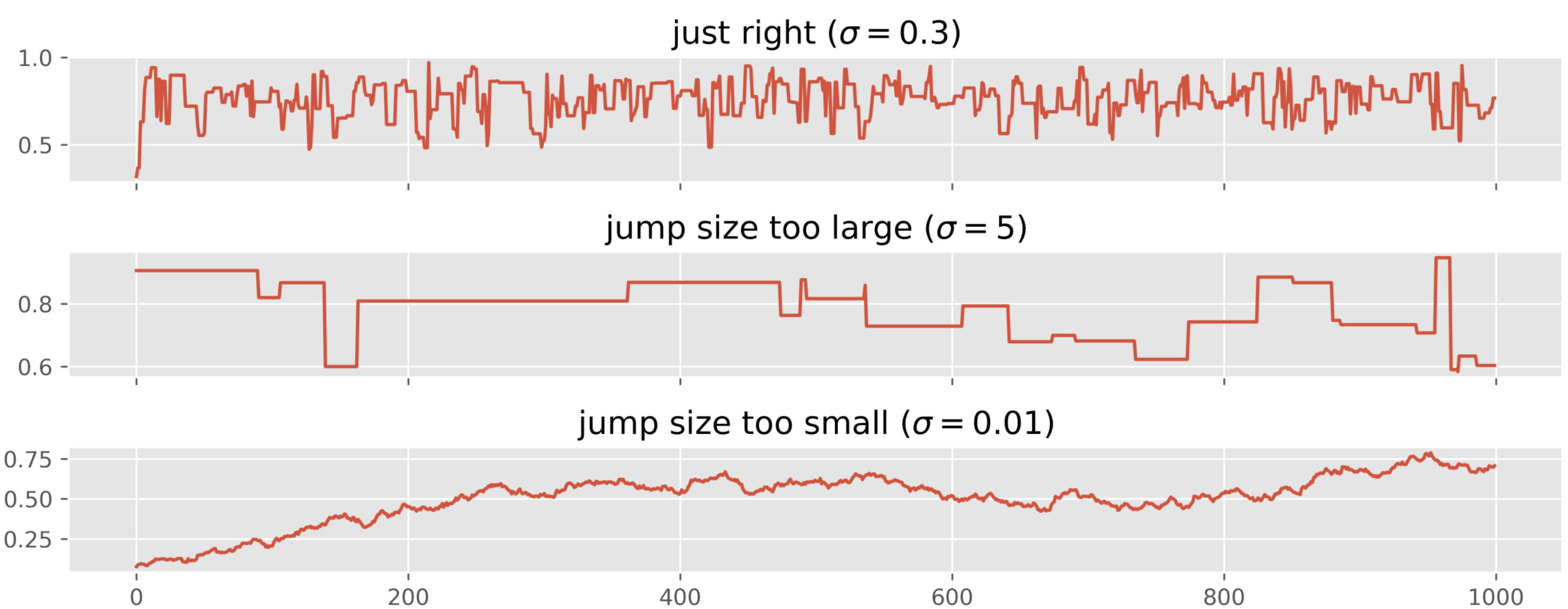
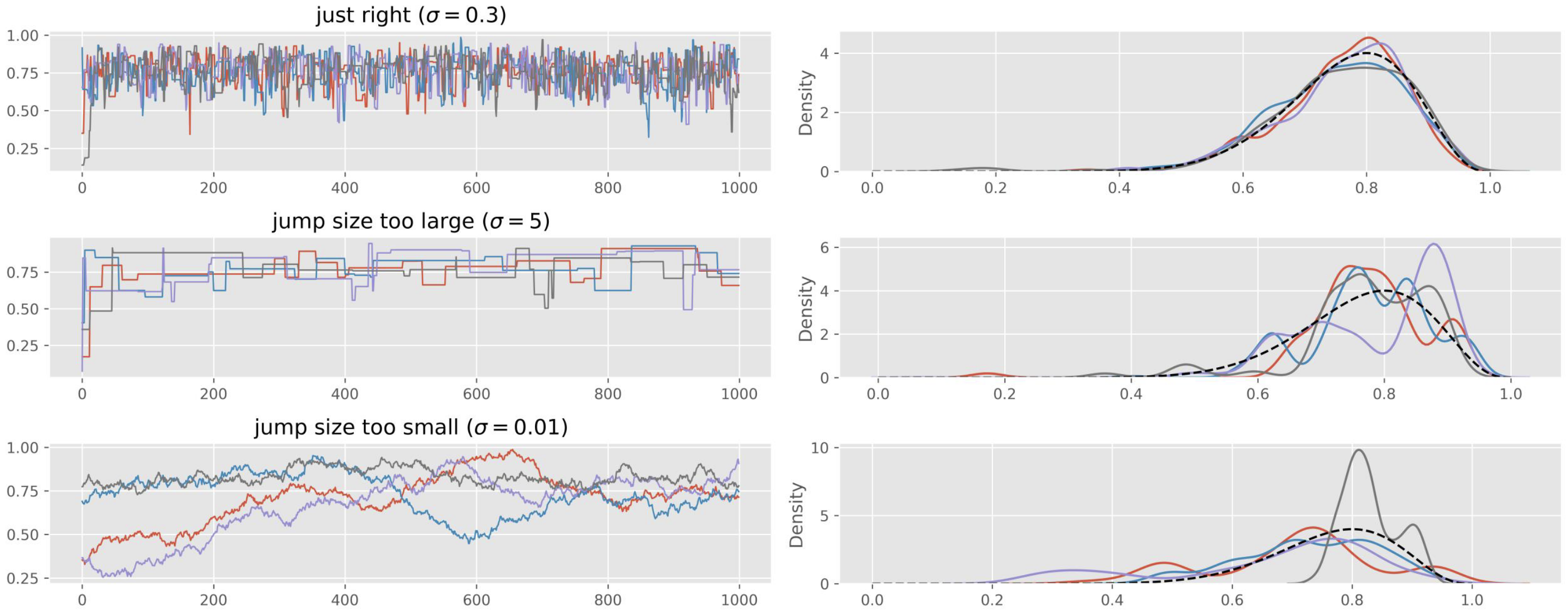
For Metropolis specifically, problematic trace plots often indicate: Proposal variance too small (tiny steps, high acceptance, poor exploration). Proposal variance too large (proposals rejected, chain rarely moves). Tunable by adjusting .
Notebook Cell
import arviz as az
az.plot_trace(trace, kind='trace', figsize=(12, 3))
plt.show()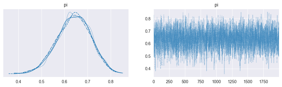
Chains explore the same region (“fuzzy caterpillars”)
No systematic upward or downward drift.
No chains stuck in a narrow band.
Different chains overlap well.
Run multiple chains: Posterior histograms or kernel density estimates for each chain separately
Distributions from all chains almost perfectly overlap.
No unique behavior in one chain.
Autocorrelation plots: Autocorrelation function (ACF) of each chain as a function of lag
Source
import arviz as az
import matplotlib.pyplot as plt
az.plot_autocorr(trace, max_lag=30, figsize=(12, 3))
plt.show()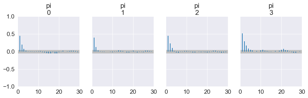
Autocorrelation decays quickly with lag.
Very slow decay or persistent high correlation means poor mixing and low effective sample size.
Rank plots / rank bars: For each parameter, pool all samples from all chains, compute their ranks, then see how ranks are distributed per chain (as in ArviZ’s rank plots)
Source
import arviz as az
import matplotlib.pyplot as plt
az.plot_trace(trace, kind='rank_bars', figsize=(12, 3))
plt.show()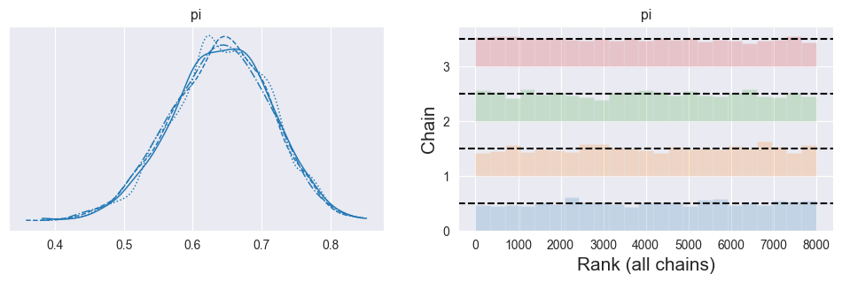
Ranks within each chain are roughly uniformly distributed.
All chains show similar, flat-ish rank patterns.
Strong deviations (U‑shape, spikes, or clearly different patterns per chain) indicate non‑convergence or poor mixing.
(R‑hat, Gelman–Rubin statistic): Compares total chain data variance (concatenated) vs. the mean variance within individual chains. Summarizes the overlaid density plots of multiple chains and provides a numerical measure for their diagreement.
Notebook Cell
trace_summary(trace)(e.g. < 1.01–1.05) means chains have likely converged to same target distribution.
means potential non‑convergence; increase iterations, needs better initialization, or reparameterization.
ESS (effective sample size): Estimates how many independent draws your autocorrelated chain is equivalent to
Notebook Cell
trace_summary(trace)ESS large relative to the number of draws, giving stable posterior summaries. Rule of thumb: ESS / N > 10%
Very small ESS (especially compared to total draws) means strong autocorrelation, poor mixing, unreliable summaries.
ess_bulk (Bulk ESS): Use this to assess reliability of posterior means, medians, and central credible intervals. Estimates the effective sample size for the central part of the distribution (around the median/mean). Interpretation: Higher is better. If ess_bulk is very small relative to the total number of draws, the chain is autocorrelated or has poor mixing in the center of the distribution.
ess_tail (Tail ESS): Use this to assess reliability of HDI/credible interval bounds and tail probabilities. Estimates the effective sample size specifically for the tails of the distribution (extreme quantiles, typically 5th and 95th percentiles). Interpretation: Higher is better. Can be substantially lower than ess_bulk if the tails are poorly explored.
Posterior Summaries, Prediction, and Uncertainty
Notebook Cell
import pymc as pm
import arviz as az

# Data: k successes out of n trials
n = 40
k = 26

with pm.Model() as model:
    pi = pm.Beta("pi", alpha=1.0, beta=1.0)  # Prior on probability pi
    y = pm.Binomial("y", n=n, p=pi, observed=k) # Likelihood
    trace = pm.sample( # Sample posterior
        draws=2000,
        tune=1000,
        chains=4,
        target_accept=0.9,
        random_seed=42
    )

az.plot_posterior(trace, hdi_prob=0.80) # Posterior plot: shows density + HDI interval + mean
trace_summary(trace, hdi_prob=0.80)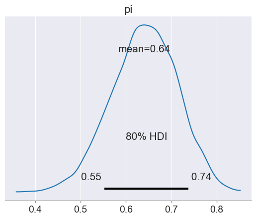
Point Summaries: Mean, Variance, Maximum A Posteriori (MAP / Posterior Mode)
Notebook Cell
stats = trace_summary(trace)
stats # Use `stats.loc['pi']['mean']` to access specific valuesGiven posterior samples :
Posterior mean:
Posterior variance:
Maximum A Posteriori (MAP) or Posterior Mode: ; To compute: Use closed form Posterior Mode if available; or Differentiate with respect to , set the derivative to zero, and solve for ; or use numerical optimization when there is no closed form.
Credible Intervals vs. Confidence Intervals
Source
import numpy as np
import pymc as pm
import matplotlib.pyplot as plt
from scipy.stats import beta
from statsmodels.stats.proportion import proportion_confint

pi_x = np.linspace(0, 1, 500)

# Data: k successes out of n trials
n = 40
k = 26
p_hat = k / n

# Prior parameters: Beta(1,1) -> flat
alpha_prior = 1.0
beta_prior = 1.0

# Posterior parameters
alpha_posterior = alpha_prior + k
beta_posterior  = beta_prior + n - k
pi_y = beta.pdf(pi_x, a=alpha_posterior, b=beta_posterior)

with pm.Model() as model_binom:
    pi = pm.Beta("pi", alpha=alpha_prior, beta=beta_prior) # Prior on probability pi
    y = pm.Binomial("y", n=n, p=pi, observed=k) # Likelihood
    trace = pm.sample( # Sample posterior
        draws=2000,
        tune=1000,
        chains=4,
        target_accept=0.9,
        random_seed=42
    )

stats = trace_summary(trace, hdi_prob=0.95, var_names=['pi'])
ci_low, ci_high = proportion_confint(k, n, alpha=0.05)

# print(f"Posterior mean (pi)                  = {stats.loc['pi']['mean']:.4f}")
# print(f"Bayesian credible interval (HDI)     = {[stats.loc['pi']['hdi_low'], stats.loc['pi']['hdi_high']]}")
# print(f"Frequentist confidence interval (CI) = {[ci_low, ci_high]}")

plt.figure(figsize=(7, 4))

# Posterior density
def plot_density(x, y, label, color='darkgreen'):
    plt.plot(x, y, label=label, lw=2, color=color)
    plt.fill_between(x, y, alpha=0.2, color=color)
plot_density(pi_x, pi_y, label="Posterior density")

# Shade Bayesian credible interval (HDI)
plt.axvspan(stats.loc['pi']['hdi_low'], stats.loc['pi']['hdi_high'], color="green", alpha=0.2, label="Bayesian credible interval (HDI)")

# Mark frequentist CI as a horizontal bar at y=0
plt.hlines(y=0.0,xmin=ci_low,xmax=ci_high,colors="red",linewidth=4,label="Frequentist confidence interval (CI)")

# Mark posterior mean and p_hat
plt.axvline(stats.loc['pi']['mean'], color="k", linestyle="--", label="Posterior mean")
plt.axvline(p_hat, color="blue", linestyle="--", label="Sample proportion $\hat p$")

plt.xlim(0, 1)
plt.xlabel(r"$\pi$")
plt.ylabel("density")
plt.title("Posterior density with Bayesian credible interval vs frequentist CI")
plt.legend(loc="upper left", fontsize=9)
plt.tight_layout()
plt.show()
Credible interval (Bayesian): For posterior , an 80% credible interval satisfies: . It’s a direct statement about the parameter: “Given data and model, we believe with 80% plausibility that lies in .”
HDI (Highest Density Interval): Among all 80% intervals, choose the one where posterior density is everywhere at least as high as outside. It minimizes width for a given mass; It contains the most probable values by construction.
Confidence interval (frequentist): 80% CI: in 80% of repeated experiments, the interval constructed by a given procedure will contain the fixed true . It does not allow the statement “ is in this specific interval with probability 0.8”.
Aleatoric vs. Epistemic Uncertainty
Law of total variance:
Aleatoric Uncertainty: irreducible data noise (e.g. binomial or Gaussian observation noise).
Epistemic Uncertainty: uncertainty about model parameters; reducible with more/better data.
If Epistemic is bigger than Aleatoric, it means collecting more data can meaningfully reduce predictive uncertainty.
If Aleatoric is bigger than Epistemic, it means that even infinite data cannot substantially reduce predictive spread (inherent randomness).
Notebook Cell
uncertainty_summary(trace.posterior, family='binominal', n=n, var_name='pi')
# uncertainty_summary(trace.posterior, family='normal', mu='mu', sigma='sigma')
# uncertainty_summary(trace.posterior, family='poisson', var_name='lambda')Notebook Cell
# Double check with posterior predictive:

var_name = 'y'
with model:
    predictions = pm.sample_posterior_predictive(trace, var_names=[var_name], random_seed=42)
predictive_var = predictions.posterior_predictive[var_name].var(ddof=1).values

print(f"Predictive Variance = {predictive_var} (for {predictions.posterior_predictive.y.values.size} samples)")
trace_summary(predictions.posterior_predictive, var_names=[var_name])Predictive Variance = 17.244173631078883 (for 8000 samples)
Hypothesis Testing
Many branches of science depend on hypothesis testing to build knowledge. Hypothesis tests are often used for feature selection (e.g. t-test p-value for features in frequentist linear regression). In Bayesian statistics, one method for model selection is based on hypothesis testing (a model is a hypothesis).
Frequentist vs. Bayesian Hypothesis Tests
Frequentist hypothesis testing can only compute the probability of data under a given hypothesis. Set up a null hypothesis and discard it if the probability is too low. This approach is dangerous when we measure unlikely data or are looking at unlikely hypotheses.
Bayesian hypothesis testing can compute , i.e. our posterior belief in given data ! Does not need a null hypothesis - can compare any two or more competing hypotheses! Bayesian and frequentist hypothesis tests return different results whenever there is heavy prior belief in and we have measured unlikely data that are in favor of : The Bayesian approach is more robust in this case because it supports the philosophy of “one random accident should not overthrow an established theory”.
One-Sided Hypothesis Tests
Frequentist Hypothesis Test: Null Hypothesis Significance Testing (NHST)
Define and
Define an estimator and significance level (false positive rate, usually )
Define a test statistic (i.e. z-score in case of binominal distribution, type of test statistic depends on estimator!):
Determine p-value:
If , reject $
Bayesian Hypothesis Test: Compare posterior probability of hypotheses
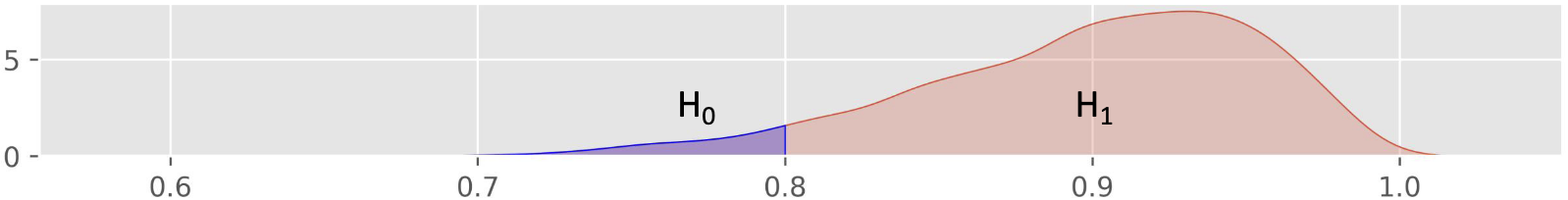
Define and :
80% of people or less in the local population are able to roll their tongue
More than 80% of people in the local population are able to roll their tongue
Define a prior distribution for (e.g. Beta(1,1) for flat prior)
Define a likelihood function (e.g. Binomial likelihood)
Sample posterior
Approximate posterior distribution of using and
pH1d = np.mean(trace.posterior.pi.values > 0.8)
pH1d, 1.0 - pH1d
Notebook Cell
# With posterior samples pi_i, approximate:
import numpy as np
import pymc as pm

# Data: k successes out of n trials
n = 40
k = 26

with pm.Model() as one_sided_model:
    # Prior on pi: flat Beta(1,1)
    pi = pm.Beta("pi", alpha=1.0, beta=1.0)

    # Likelihood
    y = pm.Binomial("y", n=n, p=pi, observed=k)

    # Sample posterior
    trace = pm.sample(
        draws=3000,
        tune=1000,
        chains=4,
        target_accept=0.9,
        random_seed=42
    )

# Extract posterior samplesd
pi_samples = trace.posterior["pi"].values.flatten()

# Posterior probability of H1: pi > 0.8
P_H1_post = np.mean(pi_samples > 0.8)
P_H0_post = 1.0 - P_H1_post

print(f"P(H1: pi > 0.8 | data)      = {P_H1_post:.3f}")
print(f"P(H0: pi ≤ 0.8 | data)      = {P_H0_post:.3f}")
print(f"Posterior odds H1:H0 = {P_H1_post / P_H0_post:.3f}")P(H1: pi > 0.8 | data) = 0.010
P(H0: pi ≤ 0.8 | data) = 0.990
Posterior odds H1:H0 = 0.010
Bayes Factor and Odds
Notebook Cell
# Prior probabilities under Beta(1,1)
P_H0_prior = 0.8
P_H1_prior = 1.0 - P_H0_prior  # P(pi > 0.8) for uniform prior = 0.2

prior_odds = P_H1_prior / P_H0_prior
post_odds  = P_H1_post / P_H0_post

BF_10 = post_odds / prior_odds

print(f"Prior Odds H1:H0            = {prior_odds:.3f}")
print(f"Posterior Odds H1:H0        = {post_odds:.3f}")
print(f"Bayes Factor BF_10          = {BF_10:.3f}")
Prior Odds H1:H0 = 0.250
Posterior Odds H1:H0 = 0.010
Bayes Factor BF_10 = 0.040
Prior odds for vs (how much more likely is than ): , flip the ratio if you are interested in how much more likely is than
Posterior odds after data:
Bayes factor , describes how much my believe changed or how much I learned from the data. Rules of Thumb: 1–3: barely worth mentioning, 3–10: substantial, 10–100: strong, bigger than 100: decisive evidence in favour of .
Two-Sided Hypothesis Tests
Region of Practical Equivalence (ROPE)
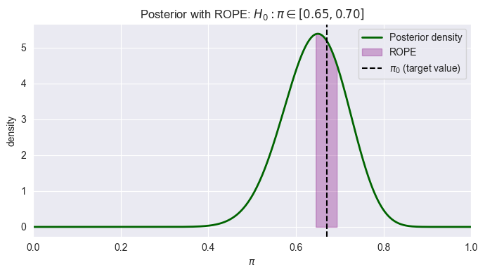
In Bayesian inference, testing whether a parameter exactly equals a specific value is statistically problematic because the probability of a continuous parameter equaling any single point is essentially zero. Instead, ROPE defines a range of values considered “practically equivalent” to the null hypothesis. For testing whether a parameter is practically equal to some value , define a ROPE, e.g. .
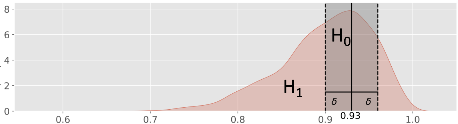
: Exactly 93% of people in the local population are able to roll their tongue for and some .
: More or less than 93% of people in the local population are able to roll their tongue outside that interval.
pi0 = 0.93; delta = 0.03
pi_values = trace.posterior.pi.values
pH0d = np.mean((pi_values > pi0 - delta) &
    (pi_values < pi0 + delta))
pH1d = 1 - pH0d
pH0d, pH1d, (pH0d / pH1d)
If most posterior mass lies inside the ROPE, you accept practical equivalence; otherwise, you conclude a meaningful difference. If the posterior distribution is fairly diffuse, with substantial mass both inside and outside this range a narrow ROPE {small ) can create an inconclusive result. A larger ROPE (bigger ) reflects what differences you actually care about practically: If you only need to know whether the true proportion is “around 93%” rather than “exactly 93%”, a wider ROPE makes sense.
Posterior Predictive Checks
Fit model and obtain posterior samples.
For each posterior draw, simulate an entire replicated dataset from the model (posterior predictive).
Compare distribution of replicated data to observed data (histograms, kernel density plots, summary statistics).
If simulated data systematically differ (e.g. lower variance, wrong tail behaviour), the model is likely misspecified (e.g. wrong likelihood family).
Source
import bambi as bmb
import pandas as pd
import numpy as np
import arviz as az
import matplotlib.pyplot as plt

data = pd.read_csv("bayesian-machine-learning/advertising.csv")
model = bmb.Model( "sales ~ TV + radio + TV:radio", data=data, family="gaussian" )
trace = model.fit(draws=2000, tune=2000, chains=4, target_accept=0.9, random_seed=42)
model.predict(trace, kind="pps")
az.plot_ppc(trace, num_pp_samples=500, figsize=(12, 3))
plt.show()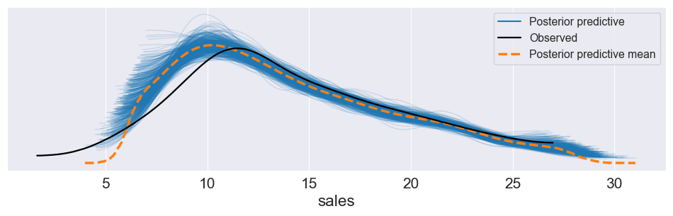
Notebook Cell
import numpy as np
import pymc as pm

# Data: k successes out of n trials
n = 40
k = 26

alpha_prior, beta_prior = 1.0, 1.0

with pm.Model() as one_sided_model:
    # Prior on pi: flat Beta(1,1)
    pi = pm.Beta("pi", alpha=alpha_prior, beta=beta_prior)

    # Likelihood
    y = pm.Binomial("y", n=n, p=pi, observed=k)

    # Sample posterior
    trace = pm.sample(
        draws=3000,
        tune=1000,
        chains=4,
        target_accept=0.9,
        random_seed=42
    )

# Extract posterior samplesd
pi_samples = trace.posterior["pi"].values.flatten()

###################################################
# Compute posterior mass in ROPE and posterior odds
###################################################

# Define ROPE
pi0 = 0.67
delta = 0.025
rope_low  = pi0 - delta
rope_high = pi0 + delta

# Posterior probabilities
P_H0_rope = np.mean((pi_samples >= rope_low) & (pi_samples <= rope_high))
P_H1_rope = 1.0 - P_H0_rope

print(f"ROPE = [{rope_low:.2f}, {rope_high:.2f}]")
print(f"P(H0: pi in ROPE | data)    = {P_H0_rope:.3f}")
print(f"P(H1: pi outside ROPE | data) = {P_H1_rope:.3f}")
print(f"Posterior odds H0:H1        = {P_H0_rope / P_H1_rope:.3f}")

#######################################
# Visualize posterior with ROPE shaded
#######################################
from scipy.stats import beta

alpha_posterior, beta_posterior = alpha_prior + k, beta_prior + n - k
pi_grid = np.linspace(0, 1, 500)
post_pdf = beta.pdf(pi_grid, a=alpha_posterior, b=beta_posterior)

plt.figure(figsize=(7, 4))

# Posterior density
plt.plot(pi_grid, post_pdf, color="darkgreen", lw=2, label="Posterior density")

# Shade ROPE region
mask_rope = (pi_grid >= rope_low) & (pi_grid <= rope_high)
plt.fill_between(pi_grid[mask_rope], post_pdf[mask_rope], color="purple", alpha=0.3, label="ROPE")

# Vertical line at pi0
plt.axvline(pi0, color="k", linestyle="--", label=r"$\pi_0$ (target value)")

plt.xlabel(r"$\pi$")
plt.ylabel("density")
plt.xlim(0, 1)
plt.title(r"Posterior with ROPE: $H_0: \pi \in [{:.2f}, {:.2f}]$".format(rope_low, rope_high))
plt.legend()
plt.tight_layout()
plt.show()ROPE = [0.65, 0.70]
P(H0: pi in ROPE | data) = 0.245
P(H1: pi outside ROPE | data) = 0.755
Posterior odds H0:H1 = 0.324
Model Checking, Selection, and Multivariate Distributions
Model selection criteria
The Fully Bayesian way: Use Bayes Factor (based on marginal likelihood). This is conceptually clean, but marginal likelihood can be hard to compute.
Use Predictive Criteria instead: These criteria trade off fit vs complexity; Bayesian evidence automatically penalizes overly complex models (“built-in Occam’s razor”).
RMSE, MAE (point prediction error using posterior predictive means)
ELPD / LOO (Expected Log Predictive Density with leave-one-out cross-validation, Computed with PSIS-LOO, higher is better)
Bayesian for regression
Bayesian Linear Regression
What is the posterior distribution of the linear regression parameters , , and ? Use Bayes’ theorem (and condition on ):
Likelihood: — probability of observing the data given parameters
Prior: — treat parameters as independent, no direct dependence on
Evidence: — marginal likelihood computed via MCMC
Then define priors and likelihood distributions:
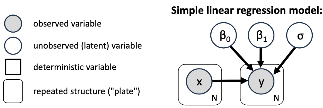
Probabilistic Graphical Model Notation
Compact graphical way to describe a model without the distributions of the individual variables. Every unobserved variable that has no arrows going into it does need a prior. Bayesian inference will get us probability distributions for the unobserved variables.
Implementation and interpretation (PyMC/Bambi)
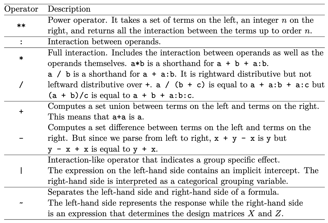
Built-in Bambi Operators
Notebook Cell
import bambi as bmb
import pandas as pd
import arviz as az
Notebook Cell
data = pd.read_csv("bayesian-machine-learning/bodyfat.csv")
model = bmb.Model("BodyFat ~ 1 + BMI",
          data=data, family="gaussian")
trace = model.fit(draws=1000, tune=1000)
trace_summary(trace, hdi_prob=0.95)Notebook Cell
az.plot_posterior(trace, hdi_prob=0.95)
plt.show()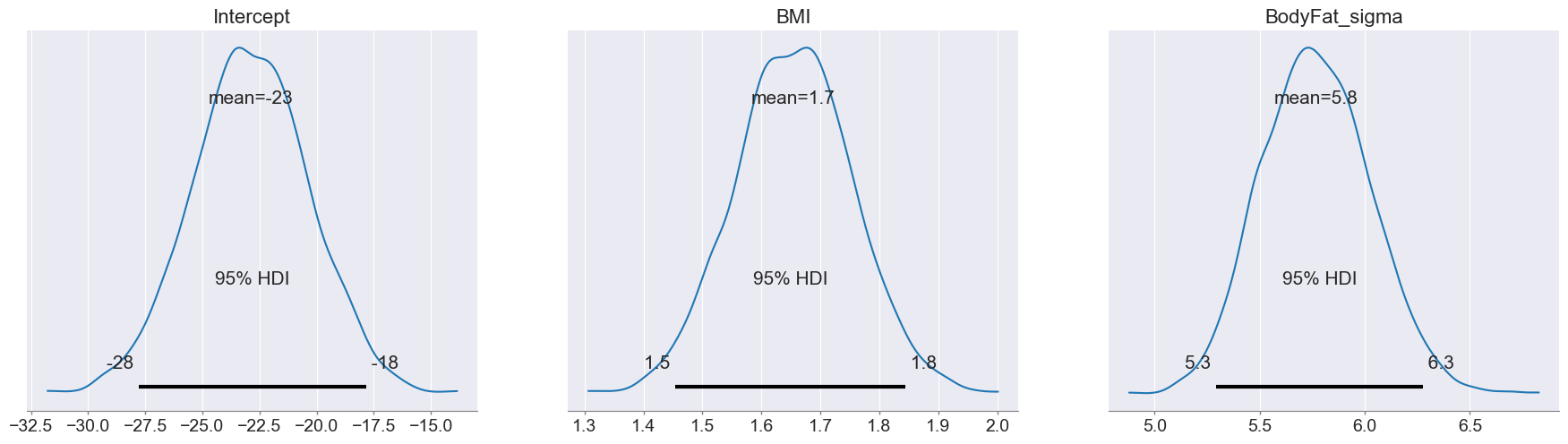
Notebook Cell
data.plot.scatter(x='BMI', y='BodyFat')
bmb.interpret.plot_predictions(
    model, trace, 'BMI', ax=plt.gca())
plt.show()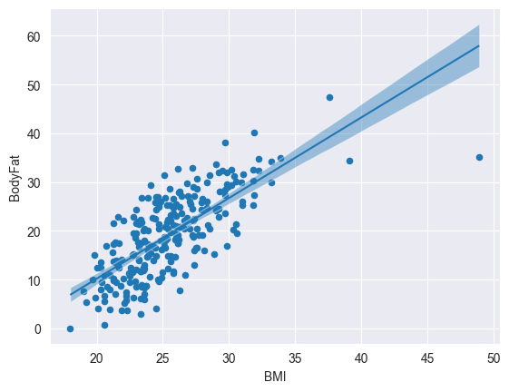
Notebook Cell
# predict out-of-sample data. for in-sample remove `data=...`
predictions = model.predict(trace, data=pd.DataFrame({ 'BMI': [20, 30, 50] }), kind="pps", inplace=False)
uncertainty_summary(predictions.posterior, family='normal', mu='BodyFat_mean', sigma='BodyFat_sigma')Notebook Cell
predictions.posterior_predictive.BodyFat.var().values # double check posterior predictive variancearray(463.07425281)Robust Linear Regression
Motivation: Outliers can have a big impact on the resulting regression line.
Reason: The Gaussian likelihood does not like points far away from its center.
Solution: Can be mitigated using a Student’s t-distribution with a heavier tail. Bayesians often prefer to change the likelihood instead of the data because its more reproducible.
model_robust = bmb.Model("BodyFat ~ BMI",
                    data=data, family="t")
trace_robust = model.fit(draws=1000, tune=1000)
trace_summary(trace_robust, hdi_prob=0.95)
Output
Gaussian Processes (GPs)
Intuition and definition
Gaussian Processes are prior distributions over functions: . A Gaussian Process is fully characterized by: Mean and a Covariance function
Covariance function must be: Symmetric and Positive semi-definite: for any finite set of inputs, the matrix must produce non-negative quadratic forms . If using a “kernel” that is not positive semi-definite (e.g. ), you can obtain negative predictive variances in the formula . Such a function is not a valid covariance function, because a covariance matrix must be positive semi-definite, implying predictive variance must be .
Key Intuition about Gaussian Processes: If things are close to each other, they should behave similar (i.e. be stronger correlated). That implies that the covariance between outputs is given in terms of the inputs.
Conditioning Rule: (“whats the prediction given the training data”)
Posterior Distribution for given , including observation noise:
Inverting the covariance matrix of the noisy observations is the most computationally expensive step, resulting in a complexity of . Therefore, large datasets are challenging for standard GPs.
GP regression: predictive mean and variance
Notebook Cell
import pandas as pd
import matplotlib.pyplot as plt
from sklearn.gaussian_process.kernels import RBF, WhiteKernel
from sklearn.gaussian_process import GaussianProcessRegressor
from sklearn.model_selection import train_test_split

length_scale = 300.0
variance = 100.0
sigma_obs = 80  # observation noise std

df = pd.read_csv("bayesian-machine-learning/credit_data.csv")
X_train, X_test, y_train, y_test = train_test_split(
    df[['Balance']],
    df[['Limit']],
    test_size=0.2,      # 20% test, 80% train
    random_state=42,    # for reproducibility
    shuffle=True        # default; set False if time series
)

kernel = variance * RBF(length_scale=length_scale) + WhiteKernel(noise_level=sigma_obs**2)
gpr = GaussianProcessRegressor(kernel=kernel, alpha=0.0, optimizer=None, normalize_y=False)
gpr.fit(X_train, y_train)

X_plot = np.linspace(X_test["Balance"].min(), X_test["Balance"].max(), 400).reshape(-1, 1)
y_mean, y_std = gpr.predict(X_plot, return_std=True)

# ---- Plot ----
plt.figure(figsize=(8, 5))

# Training and test points
plt.scatter(X_train["Balance"], y_train, color="k", alpha=0.6, label="train")
plt.scatter(X_test["Balance"],  y_test,  color="gray", alpha=0.6, label="test")

# GP mean and 95% interval
plt.plot(X_plot[:, 0], y_mean, color="C0", lw=2, label="GP mean")
plt.fill_between(
    X_plot[:, 0],
    y_mean - 1.96 * y_std,
    y_mean + 1.96 * y_std,
    color="C0",
    alpha=0.2,
    label="95% CI"
)

plt.xlabel("Balance")
plt.ylabel("Limit")
plt.title("Gaussian Process Regression")
plt.legend()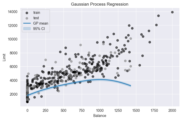
Predictive distribution for response :
Training outputs .
Covariance matrix for training outputs (including noise):
Covariances between test point and training points:
Prior variance at test point (for ):
Connection to kernels and PSD requirement
Common kernels and hyperparameters:
Squared Exponential / RBF: , (: output variance, : length scale (smoothness))
Matérn (controls differentiability via ):
Rational Quadratic (mixture over length scales).
Bayesian Networks and Causal Inference
Structural Causal Models (SCMs) and Bayesian Networks
SCM formalism (from BN lecture notes):
Endogenous (ovservered) variables : determined by structural equations.
Exogenous (unobserved) variables : external noise.
Structural equations: each variable is a function of its parents (endogenous causes) and noise (exogenous causes):
Joint distribution defined via and structural equations.
A Bayesian Network (BN) is a DAG over variables such that joint distribution factorizes as:
Graph encodes conditional independencies.
Each node has a Conditional Probability Table (CPT) or parameterized distribution.
Basic graph motifs and conditional independence
Three canonical patterns:
Chain (serial):
and correlated marginally.
Conditional independence given the middle node: .
Fork (common cause):
and correlated marginally (through common cause ).
Conditional independence given cause: .
Collider (v‑structure):
and independent marginally.
Conditioning on collider (or its descendants) induces dependence (explaining away).
Explaining away: In collider , observing the effect makes causes and compete.
Example: “Smoker” and “Covid” both cause “Hospitalization”; given hospitalization, learning that patient is a smoker reduces belief that Covid is cause, and vice versa.
Computing Probabilities from Joint Tables
Given full joint distribution table :
Marginal:
Conditional:
Example:
Interventions and the do‑operator
Conditioning: describes correlations in observed data; may itself be caused by other variables (confounded).
Intervention: describes what happens if we force to (surgery on the graph):
All incoming edges into are cut.
is set externally.
The rest of the graph and conditional distributions remain unchanged.
For a treatment , outcome , and set of observed confounders that block all backdoor paths (backdoor criterion), adjustment formula:
Expectation Maximization (EM)
The EM algorithm iteratively maximizes the log-likelihood of the observed data. is hidden, is observed.
Initialize randomly
Repeat until convergence:
E-step:
Compute for each (probabilistic inference)
Create fully-observed weighted examples: with weight
M-step:
Perform maximum likelihood (count and normalize) on weighted examples to update